All in One View
Content from Introduction to the LaTeX Workflow
Last updated on 2026-04-08 | Edit this page
Overview
Questions
- What do I need to do to write and edit a LaTeX document?
- How can I render a LaTeX document?
Objectives
- Demonstrate how to create a new LaTeX Document.
- Become familiar with the TeXworks interface.
- Compile a LaTeX document with the TeXworks editor.
- Compile a LaTeX document with the command line.
What is LaTeX
LaTeX is a typesetting language, useful for combining text with mathematical equations, figures, tables, and citations, among other things.
Unlike common word processors like Microsoft Word or LibreOffice Writer, LaTex is a markup language, meaning that formatting (including bold text, bullet points, and changes in font size) is indicated by the use of commands, special characters, or environments.
In order to produce the actual document, this mark-up text must be compiled. Errors in the mark-up can either be non-fatal, meaning the document will compile with some warnings; or fatal, meaning the document will fail to compile.
Our First LaTeX Document
To begin with, we will create a new directory to hold our files for
this workshop. Call it latex-workshop, and make a note of
the path to this directory.
Start the TeXworks editor and immediately “save” the file. This will
prompt you for a location to save the file, so navigate to the
latex-workshop directory you just created, and save the
file as main.tex.
The Interface
The TeXStudio interface is divided into several sections: - The Editor: This is where you write your LaTeX code. It supports syntax highlighting and basic code completion. - The Preview Pane: This shows the compiled output of your LaTeX code. This window will appear whenever we compile the document. - The Menu Bar: This contains various options for managing your document, such as saving, compiling, and printing. You can also access the preferences and settings from here. - The Toolbar: This contains buttons for common actions, such as saving, compiling, and inserting common LaTeX commands. - The Status Bar: This shows information about the current document, such as the line and column number, the current compiler, and any warnings or errors that may have occurred during compilation.

The TeXworks interface is divided into three main sections: - The Editor: This is where you write your LaTeX code. It supports syntax highlighting and basic code completion. - The Preview Pane: This shows the compiled output of your LaTeX code. This window will appear whenever we compile the document. - The Menu Bar: This contains various options for managing your document, such as saving, compiling, and printing. You can also access the preferences and settings from here.
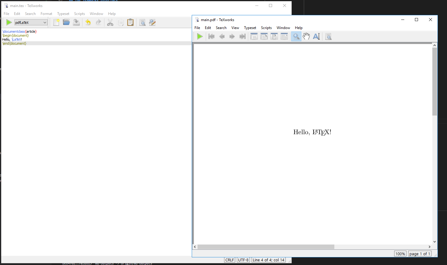
The overall interface is designed to be simple and intuitive, focusing on the essential features of a LaTeX editor. Note the large green triangle button in the top left corner of the interface. This is the “Typeset” button, which compiles your LaTeX document and updates the preview pane with the rendered output. Next to the “Typeset” button is a drop-down menu that allows you to select the typesetting engine you wish to use. For this workshop, we will use the default engine, PDFLaTeX.
Compiling a LaTeX Document
Type the following code into the editor:
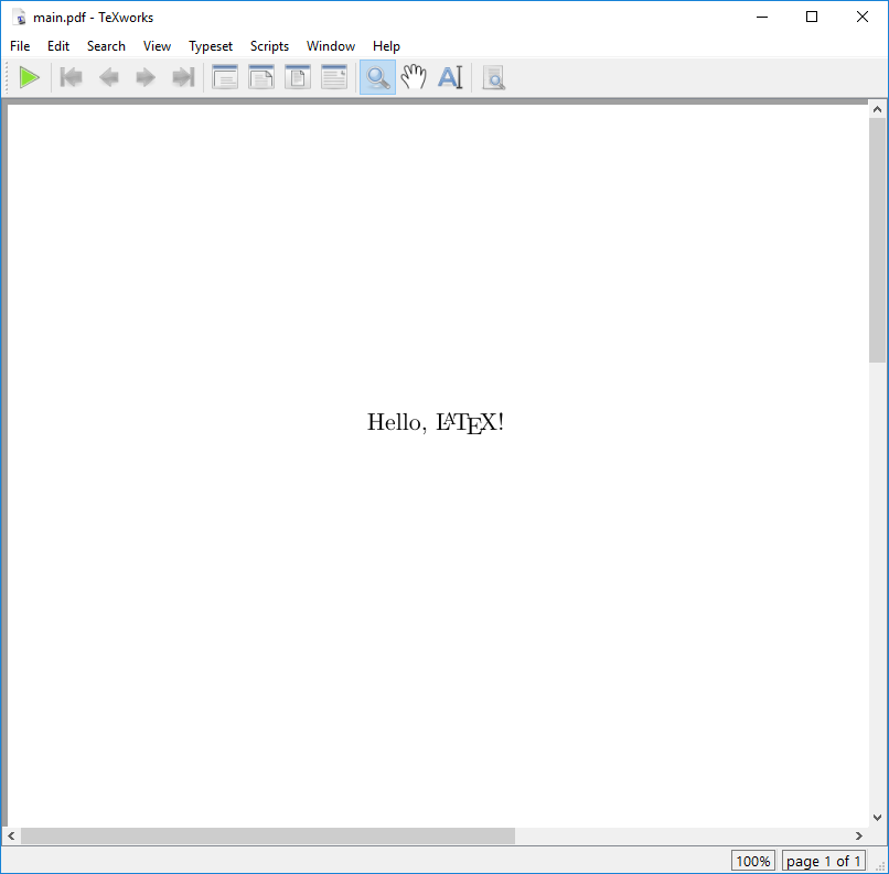
Now click the green “Typeset” button in the top left corner of the interface. This will compile the document and update the preview pane with the rendered output. You should see a PDF preview of the document with the text “Hello, LaTeX!”.
When you click the “Typeset” button, the editor will run the LaTeX compiler on your document. You will see a window appear on the bottom of the interface called “Console output”. This window contains the output of the compiler, including any warnings or errors that may have occurred during the compilation process. We will talk about this in more detail in a later episode.
Compiling a LaTeX Document from the Command Line
Using an IDE like TeXStudio or TeXworks is a convenient way to write and compile LaTeX documents, but you are not limited to using it. Any program that can edit text files can be used to write LaTeX, which we can then compile from the command line.
You can use any text editor to write your LaTeX code. Some popular text editors for LaTeX include:
- Visual Studio Code
- Emacs
- Vim
- Notepad++ (Windows only)
We will continue to demonstrate with TeXworks, but you can use any text editor you prefer.
To compile a LaTeX document from the command line, you can use the
pdflatex command. Open a console or terminal window, then
navigate to the directory where you saved your main.tex
file.
Useful commands for navigating the command line:
-
cd <directory>: Change directory to<directory>. -
ls(Linux/macOS) ordir(Windows): List the files in the current directory. -
pwd(Linux/macOS): Print the current working directory.
Once you are in the correct directory, run the following command:
You should see output similar to the following:
This is pdfTeX, Version 3.141592653-2.6-1.40.28 (TeX Live 2025) (preloaded format=pdflatex)
 restricted \write18 enabled.
entering extended mode
(./main.tex
LaTeX2e <2024-11-01> patch level 2
L3 programming layer <2025-04-29>
(e:/texlive/2025/texmf-dist/tex/latex/base/article.cls
Document Class: article 2024/06/29 v1.4n Standard LaTeX document class
(e:/texlive/2025/texmf-dist/tex/latex/base/size10.clo))
(e:/texlive/2025/texmf-dist/tex/latex/l3backend/l3backend-pdftex.def)
(./main.aux)
[1{e:/texlive/2025/texmf-var/fonts/map/pdftex/updmap/pdftex.map}] (./main.aux)
)<e:/texlive/2025/texmf-dist/fonts/type1/public/amsfonts/cm/cmr10.pfb><e:/texli
ve/2025/texmf-dist/fonts/type1/public/amsfonts/cm/cmr7.pfb>
Output written on main.pdf (1 page, 21048 bytes).
Transcript written on main.log.
You can also use the compiler LuaLaTeX which is more powerful but might take a little bit longer to generate the pdf.
The output is this:
This is LuaHBTeX, Version 1.22.0 (TeX Live 2025)
 restricted system commands enabled.
(./main.tex
LaTeX2e <2025-06-01> patch level 1
L3 programming layer <2025-07-11>
 (/usr/local/texlive/2025/texmf-dist/tex/latex/base/article.cls
Document Class: article 2025/01/22 v1.4n Standard LaTeX document class
(/usr/local/texlive/2025/texmf-dist/tex/latex/base/size10.clo))
(/usr/local/texlive/2025/texmf-dist/tex/latex/l3backend/l3backend-luatex.def)
No file main.aux.

[1{/usr/local/texlive/2025/texmf-var/fonts/map/pdftex/updmap/pdftex.map}]
(./main.aux))
 406 words of node memory still in use:
   3 hlist, 1 vlist, 1 rule, 2 glue, 3 kern, 1 glyph, 4 attribute, 48 glue_spec
, 4 attribute_list, 1 write nodes
   avail lists: 2:38,3:4,4:1,5:26,6:2,7:56,9:24
</usr/local/texlive/2025/texmf-dist/fonts/opentype/public/lm/lmroman7-regular.o
tf></usr/local/texlive/2025/texmf-dist/fonts/opentype/public/lm/lmroman10-regul
ar.otf>
Output written on main.pdf (1 page, 4850 bytes).
Transcript written on main.log.
Notice how the size of the pdf is about one forth when compiling with LuaLaTeX compared to pdflatex.
In the directory where you ran the command, you should now see a new
file called main.pdf, as well as some other files that were
created during the compilation process. The main.pdf file
is the rendered output of your LaTeX document, and you can open it with
any PDF viewer to see the result.
When you looked in your directory, you may have noticed that several
other files were created in addition to the main.pdf file.
These files are:
-
main.aux: This file contains auxiliary information used by LaTeX during the compilation process, such as cross-references and citations. -
main.log: This file contains the log output of the LaTeX compiler, including any warnings or errors that occurred during the compilation process.
The main.aux file is not something we really need to
worry about at this point, but the main.log file can be
useful for debugging if you encounter any issues with your LaTeX
document. We’ll take a closer look at the log file in a later
episode.
Challenge 1: NEED A NEW CHALLENGE
Challenge 3: NEED A NEW CHALLENGE
- We can use the TeXworks editor to write and compile LaTeX documents.
- The TeXworks interface is divided into three main sections: the editor, the preview pane, and the menu bar.
- We can compile a LaTeX document by clicking the “Typeset” button in the TeXworks editor.
- We can also compile a LaTeX document from the command line using the
pdflatexorlualatexcommand.
Content from Basic LaTeX Document Components
Last updated on 2026-04-08 | Edit this page
Overview
Questions
- What is the basic structure of a LaTeX document?
- How do I see what my LaTeX document looks like when it’s rendered?
Objectives
- Become familiar with the basic structure of a LaTeX document.
- Use TeXworks to render a LaTeX document into a PDF.
- Identify how to add special characters to a LaTeX document.
Editing the Document
We can edit the main.tex file with TeXworks (or any text
editor of your choice). Let’s start by creating a simple LaTeX
document:
LATEX
\documentclass{article}

\begin{document}
Hello World!

This is my first LaTeX document.
\end{document}
Errors happen! Check that you have entered each line in the text file exactly as written above. Sometimes seemingly small input changes give large changes in the result, including causing a document to not work. If you are stuck, try erasing the document and copying it fresh from the lines above.
Looking at our document
Our first document shows us the basics. LaTeX documents are a mixture of text and commands.
-
Commands start with a backslash
\and sometimes have arguments in curly braces{}. - Text is what you want to appear in the document and requires no special formatting.
Let’s look at the commands we’ve used so far:
-
\documentclass{article}: This command tells LaTeX what kind of document we are creating. (We might also use this command to instruct LaTeX to use a specific font size, paper size, or other document settings - more on this later!) -
\begin{document}and\end{document}: These commands mark the beginning and end of the document body. These commands are required in every LaTeX document and create the document body.
You can have multiple \begin{...} and
\end{...} pairs in a single LaTeX document, but you must
have exactly as many \begin{...} commands as
\end{...} commands.
Everything before the \begin{document} command is called
the preamble. The preamble is where you set up the document,
including the document class, title, author, and any other settings you
want to apply to the entire document.
Comments
We can add comments to our document by using the %
character. Anything after the % on a line is ignored by
LaTeX. As in any other programming language, comments are useful for
explaining what the code is doing. We’ll start incorporating comments
into our document going forward to explain some of the specifics of the
LaTeX code we’re writing.
As we go, you should use your version of the document to add your own comments as a way of taking notes on what you’re learning, and to act as a reference for yourself in the future!
LATEX
% This command tells LaTeX what kind of document we are creating (article).
\documentclass{article}


% Everything before the \begin{document} command is called the preamble.
\begin{document} % The document body starts here
Hello World!

This is my first LaTeX document.
\end{document}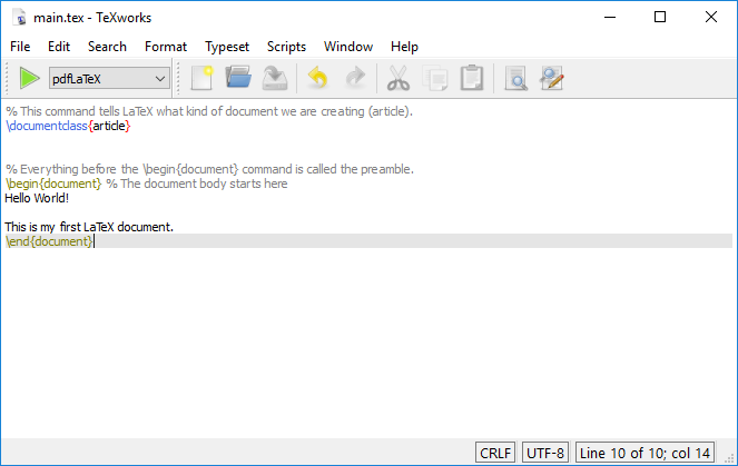
Note that the comments are displayed in a different color in the text editor. This is called “syntax highlighting”. Not all text editors will do this by default, but you can often add syntax highlighting to your text editor of choice.
Going forward, the examples we provide will not always include comments, but you should add them to your document as you see fit.
Rendering the Document
As with our example from the previous episode, we can render our
document by clicking on the large green “Typeset” button in TeXworks, or
by running the command pdflatex main.tex in our
terminal/consoloe.
When running the command in the terminal, make sure you have saved your document first, as the command will only render the last saved version of the document.
Paragraphs
Note that we have an empty line between our two lines of text. This is important in LaTeX, as this indicates a new paragraph. Let’s try removing the empty line and recompiling the document to see what happens.
You should see that the two lines of text are now displayed on the
same line. This is because LaTeX treats the two lines as part of the
same paragraph. If you want to start a new paragraph, you need to leave
a blank line between the two paragraphs. Instead of using an empty line,
there is also the command \par that leads you to the same
result of creating a new paragraph. More on this in one of the
challenges below.
Special Characters
You’ve probably noticed by now that the characters \,
{, and } are special characters in LaTeX.
There are others though, such as $, %,
&, # and ^. These characters
tend to be much less common in text, but you can use them by “escaping”
them with a backslash. For example,
-
\%produces% -
\&produces& -
\#produces# -
\^produces^
and so on.
What about the \ character?
The \ character is used to escape other characters in
latex, so it’s not possible to escape it in the same way. Instead, you
can use \textbackslash to produce a backslash in your
document.
Sometimes, special characters can, unintentionally, conflate with
characters that are used after that special character. You can prevent
that by typing {} directly behind your special character.
The following LaTeX code gives you an example:
Challenges
Challenge 1: What’s wrong with this document?
There is an error in the following LaTeX document. Can you find it?
(Feel to make a new .tex file in a new project folder to test this out!)
Each section of a LaTeX document must be enclosed in a pair of
\begin{...} and \end{...}. This document is
missing the \begin{document} command.
Challenge 2: Displaying Special characters.
How would I display the following text in a LaTeX document?
5 is greater than 3 & 2 is less than 4. This is 100% true.Challenge 3: Paragraphs with
\par.
In the section about Paragraphs from above we learned that empty
lines are important to create paragraphs. However, there is also a LaTeX
command called \par which might be of help for us. Consider
the LaTeX code below. Can you already guess which of these options
prints Hello World! and This is my first LaTeX
document. in two separate lines? (Feel to make a main.tex file in a
new project folder to test this out!)
LATEX
% This command tells LaTeX what kind of document we are creating (article).
\documentclass{article}

% Everything before the \begin{document} command is called the preamble.
\begin{document} % The document body starts here
% Option A
Hello World!

This is my first LaTeX document.

% Option B
Hello World! This is my first LaTeX document.

% Option C
Hello World! \par This is my first LaTeX document.

% Option D
Hello World! \par

This is my first LaTeX document.
\end{document}The command \par initiates a new paragraph for us even
if we write text in just one line (see Option C). Solely, Option B out
of all four options does not create the intended new paragraph as
neither an empty line nor \par is used. Moreover, Option D
gives us the same result as Option A and Option C, although we used
both, \par and an empty line.
Challenge 4: One line of code with paragraphs and special characters.
How would I display the following text in a LaTeX document but using just one line of code?
Hello World! This is my first LaTeX document.
Now, I know how to initiate paragraphs without an empty line.
Even more, I can write # and ^ correctly using LaTeX.We need to use \par to initiate a new paragraph without
using a new line of code. Moreover, we need to use escapes before each
of the special characters. The following LaTeX code will display the
text correctly:
- The
%character is used to add comments to a LaTeX document. - LaTeX documents are a mixture of text and commands.
- Commands start with a backslash
\and sometimes have arguments in curly braces{}. - We can view errors by either clicking on the “Logs and output files” or hovering over the red circle in the text editor.
After this episode, here is what our LaTeX document looks like:
Content from Error Handling
Last updated on 2026-04-08 | Edit this page
Overview
Questions
- What do I do when I get an error message?
Objectives
- Understand how to interpret error messages in LaTeX
- Learn how to fix common errors in LaTeX documents
Error Handling
Error messages in LaTeX can often be difficult to understand, especially if you’re new to the language. However there are a few common errors that we can learn to recognize and fix, and a few techniques we can use to debug our documents based on the error messages we receive.
Inevitably, everyone makes mistakes when writing LaTeX documents. When you recompile your document, you might not see any changes in the preview pane. This could be because there is an error in your document. If there is an error, you will see a red number next to the “Recompile” button over the “Logs and output files” button. You will also see certain lines highlighted in red in the text editor, along with a suggestion of what the error might be.
Let’s introduce an error into our project to see what this might look
like. Let’s introduce a typo into the documentclass command
by changing it to documnetclass. When we recompile the
document, we can see our errors:
LATEX
% This command is misspelled on purpose to generate an error
\documnetclass{article}

\begin{document}
Hello World!

This is my first LaTeX document.
\end{document}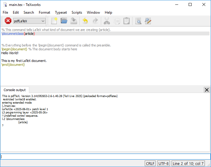
The greens triangle we clicked on is now a red octagon, indicating that there is an error. There’s also now a second tab that we can see in the editor pane now, called “Errors, warnings, badboxes”. Clicking on this tab shows us something like this:
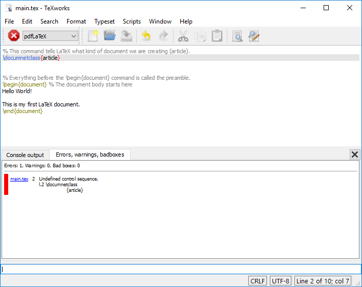
! Undefined control sequence.
l.2 \documnetclass
                  {article}
Back in the “Console Output” tab, there’s a “?”, indicating that the console is waiting for us to give it some input.
Let’s type
! LaTeX Error: Missing \begin{document}.

See the LaTeX manual or LaTeX Companion for explanation.
Type  H <return>  for immediate help.
 ...

l.2 \documentclass{article}
Keep hitting
If we run the command pdflatex main.tex in the terminal,
we will see an error message:
The text in the terminal tells us that there is an error in the
main.tex file on line 2, and that the command
\documnetclass is undefined.
Keep hitting
Once we reach the end of the error messages, we can also open the
main.log file in the project to see a full log of the
errors and warnings that were generated during the compilation.
Commands in the console:
- Type
to proceed, - S to scroll future error messages,
- R to run without stopping
- Q to run quietly,
- I to insert something
- E to edit your file
- 1 or … or 9 to ignore the next 1 to 9 tokens of input,
- H for help
- X to quit
Fixing Errors
In general, the first error message you see is the most important one
to fix. In this case, all of the subsequent errors are related to the
initial error, which is that the \documentclass command is
undefined. Once we fix the typo in the \documentclass
command, the document will compile successfully.
The subsequent errors, talking about “missing begin document”, and “font size command not defined” are all cascading errors from the initial error. When LaTeX encounters an error, it can’t continue to compile the document, so it stops and reports the error it found. This can sometimes lead to multiple error messages, but generally it’s important to fix the first error first, as this will often resolve subsequent errors.
Anatomy of an Error Message
Let’s take a closer look at one of them and see what it tells us.
! Undefined control sequence.
l.2 \documnetclass
                  {article}
This message tells us a few things: 1.
! Undefined control sequence.: This indicates that LaTeX
encountered a command that it doesn’t recognize. In this case, it’s the
misspelled \documnetclass command. 2. l.2:
This tells us that the error occurred on line 2 of the document. 3.
\documnetclass: This is the command that caused the error.
LaTeX doesn’t recognize this command because it is misspelled.
Of course, we know what the error was, so we can just fix it by
changing \documnetclass back to
\documentclass.
In general, the first error message in the list is the most useful one to look at. The other error messages are often just a result of the first error cascading down the document, so fixing the first one will often fix the rest of them too.
Fixing Errors
As we progress through this workshop, we will point out places where we get new error messages, and discuss how to interpret and fix them.
Unidentified Control Sequence
We saw this one in our first example, but it can happen any where there is a command that LaTeX doesn’t recognize. This can happen if you misspell a command, or if you forget to include a package that defines the command, of if you try to use an incorrect command.
Here’s a quick example of this error:
LATEX
\documentclass{article}

\begin{document}

\section{My Amazing Content}

  My Amazing Content: $\alpha = \fraction{1}{(1 - \beta)^2}$

\seciton{More Amazing Content}

  Even more amazing content!

\end{document}
Attempting to compile this document results in the following error message:
! Undefined control sequence.
l.9 \seciton{More Amazing Content}
So, again, we see that the error is an “Undefined control sequence”,
and it tells us that something in line 9 is not defined. In this case,
the command \seciton is not a valid LaTeX command.
Errors vs Warnings vs Information
Not all messages are equal! LaTeX has three different types of messages:
-
Error: This is a serious issue that will prevent your document from compiling. You need to fix this before you can continue. -
Warning: This is a less serious issue that may not prevent your document from compiling, but it may cause issues with the output. You should still try to fix this, but it may not be critical. -
Information: This is just a message that provides additional information about the document. You can usually ignore this.
In Overleaf, error messages are shown in red, warnings are shown in yellow, and information messages in blue.
Challenges
Challenge 1: Identify and fix the error?
The following document contains an error. Can you identify it?
The error suggests there is something wrong with line 8.
The full error message is:
! Undefined control sequence.
<argument> -b \pm \squareroot
                              {b^2 - 4ac}
l.8 $x = \frac{-b \pm \squareroot{b^2 - 4ac}}{2a}
                                                 $
The error indicates that the command \squareroot is not
defined. We haven’t covered mathematical commands yet, but the correct
command for the square root symbol is \sqrt.
There are three errors in total:
- The document is missing the
\begin{document}command at the beginning. - The
\Sectioncommand is not defined. The correct command for a section heading is\section. - The
\textbfcommand is not properly closed. It should be\textbf{Smith et al (2020)}.
- Errors are common! Don’t be discouraged by them.
- The first error message is usually the most important one to fix.
- Read the error messages carefully, they often tell you exactly what the problem is.
Content from The Structure of a Document
Last updated on 2026-04-08 | Edit this page
Overview
Questions
- How are LaTeX documents structured?
Objectives
- Identify the different kinds of section commands in LaTeX.
- Create a list within a LaTeX document.
Sections
In a word processor, you might use headings to organize your document.In LaTeX, we’ll use the section commands:
\section{...}\subsection{...}
LaTeX will handle all of the numbering, formatting, vertical spacing, fonts, and so on in order to keep these elements consistent throughout your document. Let’s add sections to our document.
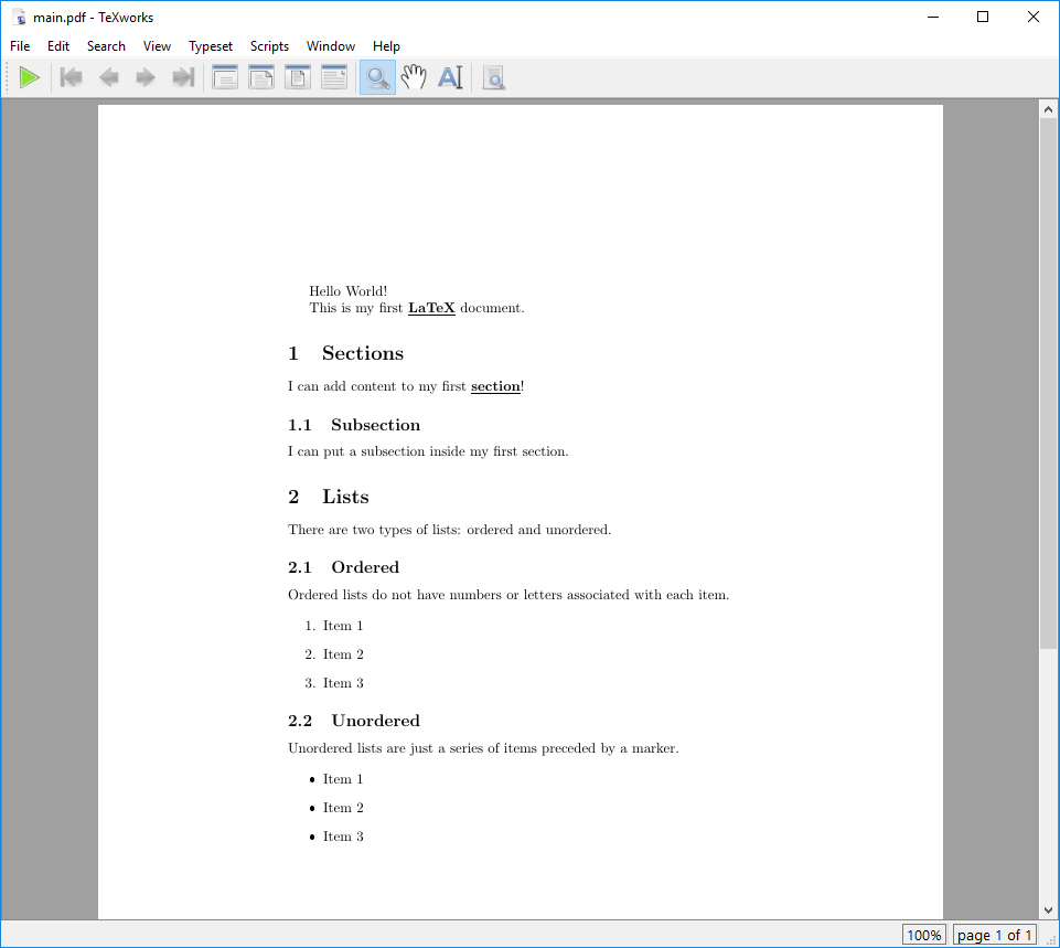
LATEX
% This command tells LaTeX what kind of document we are creating (article).
\documentclass{article}
% Everything before the \begin{document} command is called the preamble.
\begin{document} % The document body starts here
% The section command automatically numbers and formats the section heading.
\section{Sections}
Hello World!
This is my first LaTeX document.
I can add content to my first section!
% The subsection command does the same thing, but for sections within sections.
\subsection{Subsection}
I can put a subsection inside my first section.
\section{Second Section}
And this text will go into another section.
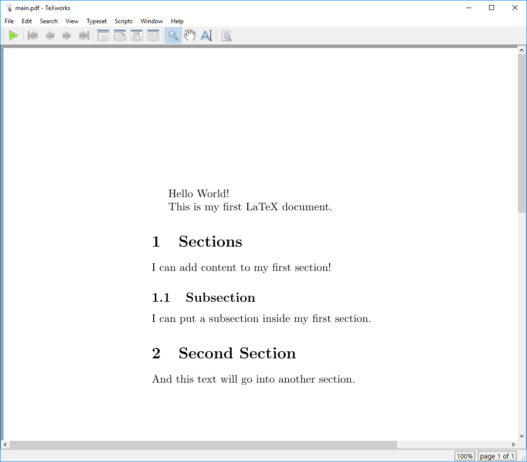
\end{document}You should have something that looks like this:
There are many different section commands in LaTeX, including
\subsubsection{...}, \paragraph{...},
\chapter{...}, and more. Each of these commands will create
a new section heading with a different level of indentation and
numbering.
Some of these commands are only available in certain document classes, so be sure to check the documentation for the class you are using.
There’s also an alternative way to create sections in LaTeX using the
\section*{...} command. This command will create a section
heading without numbering it. This can be useful for creating unnumbered
sections, such as an introduction or conclusion.
Table of Contents
We’ve seen how to make sections and how LaTeX will automatically
number them for us. But we can also use this feature to automatically
generate a table of contents for our document! We can do this by adding
the \tableofcontents command to our document body. This
will create a table of contents at the location where the command is
placed.
LATEX
% This command tells LaTeX what kind of document we are creating (article).
\documentclass{article}


% Everything before the \begin{document} command is called the preamble.
\begin{document} % The document body starts here

\tableofcontents

% The section command automatically numbers and formats the section heading.
\section{Sections}

Hello World!

This is my first LaTeX document.

I can add content to my first section!

% The subsection command does the same thing, but for sections within sections.
\subsection{Subsection}

I can put a subsection inside my first section.

\section{Second Section}

And this text will go into another section.

\end{document}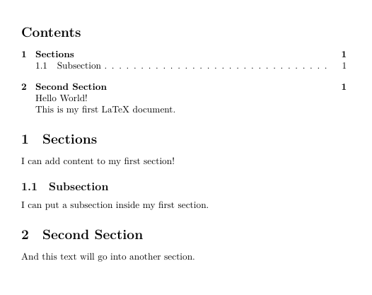
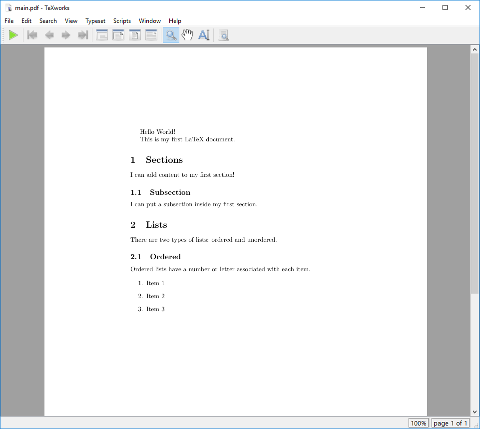
Lists
In LaTeX, as in markdown, there are two types of lists: ordered and
unordered. They are both defined with \begin{...} and
\end{...} commands, as we saw with the document body. Let’s
add an ordered list to our document.
We’ll replace our “Second Section” with one for “Lists” and add an ordered list:
LATEX
% This command tells LaTeX what kind of document we are creating (article).
\documentclass{article}


% Everything before the \begin{document} command is called the preamble.
\begin{document} % The document body starts here

\tableofcontents

% The section command automatically numbers and formats the section heading.
\section{Sections}

Hello World!

This is my first LaTeX document.

I can add content to my first section!

% The subsection command does the same thing, but for sections within sections.
\subsection{Subsection}

I can put a subsection inside my first section.

\section{Lists}

There are two types of lists: ordered and unordered.

\subsection{Ordered}

Ordered lists have a number or letter associated with each item.

\begin{enumerate}
  \item Item 1
  \item Item 2
  \item Item 3
\end{enumerate}

\end{document}
When you compile this document, you should see something like this in the preview pane:
Note that the \item commands do not need to be enclosed
in braces. These commands do not take any arguments, so they can be used
as standalone commands. The text that follows the \item
command will be treated as the content of the list item. However, you
are able to specify your own bullet point symbols with
\item[] manually. For instance, if you want a list with
small letters in brackets you can use the following LaTeX code:
LATEX
% This command tells LaTeX what kind of document we are creating (article).
\documentclass{article}


% Everything before the \begin{document} command is called the preamble.
\begin{document} % The document body starts here

% List with custom bullet point symbols
\begin{itemize}
  \item[(a)] Item 1
  \item[(b)] Item 2
  \item[(c)] Item 3
\end{itemize}

\end{document}It’s also possible to create a list with roman numerals automatically
with the enumitem package:
LATEX
\documentclass{article}
\usepackage{enumitem} %<-- package for lists https://texdoc.org/serve/enumitem/
% \setlist{label=\Roman*} %<-- globally defining the enumeration system
\begin{document}
\begin{enumerate}[
  label=\emph{\roman*}, %<-- change labeling system locally (or \Roman)
  leftmargin=5cm, %<-- change indent on the left
]
  \item First
  \item Second
  \item Third
  \item Fourth
\end{enumerate}
\end{document}
Adding an unordered list is just as easy. We can use the exact same
syntax, but replace the enumerate environment with
itemize.
LATEX
% This command tells LaTeX what kind of document we are creating (article).
\documentclass{article}


% Everything before the \begin{document} command is called the preamble.
\begin{document} % The document body starts here

\tableofcontents

% The section command automatically numbers and formats the section heading.
\section{Sections}

Hello World!

This is my first LaTeX document.

I can add content to my first section!

% The subsection command does the same thing, but for sections within sections.
\subsection{Subsection}

I can put a subsection inside my first section.

\section{Lists}

There are two types of lists: ordered and unordered.

\subsection{Ordered}

Ordered lists do not have numbers or letters associated with each item.

\begin{enumerate}
  \item Item 1
  \item Item 2
  \item Item 3
\end{enumerate}

\subsection{Unordered}

Unordered lists are just a series of items preceded by a marker.

\begin{itemize}
  \item Item 1
  \item Item 2
  \item Item 3
\end{itemize}

\end{document}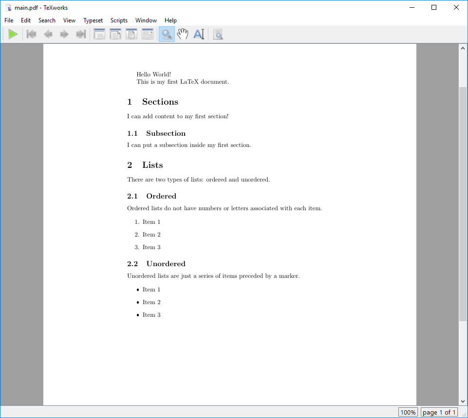
Challenges
Challenge 1: What needs to change?
Challenge 2: Can you do it?
We would like to have the following appear in our LaTeX document:
- Apples
- Gala
- Fuji
- Granny Smith
- Bananas
- Oranges
How would you write this in LaTeX?
Challenge 3: Enumerate your list manually
We would like to have the following appear in our LaTeX document:
- Gala
- Fuji
- Granny Smith
How would you write this in LaTeX without using
enumerate but itemize with
\item[]?
- LaTeX documents are structured using section commands.
- There are many different section commands in LaTeX, including
\subsubsection{...},\paragraph{...},\chapter{...}, and more. - Lists in LaTeX are created using the
enumerateanditemizeenvironments.
After this episode, here is what our LaTeX document looks like.
Content from Using Document Classes
Last updated on 2025-07-16 | Edit this page
Overview
Questions
- What is a LaTeX Document class?
- How does a document class affect the layout of a LaTeX document?
Objectives
- Identify the various types of document classes available in LaTeX
- Create a document using an alternative document class
What is a Document Class?
A document class sets up the general layout of the document, including (but not limited to):
- design (margins, fonts, spacing, etc)
- availability of chapters
- title page layout
Document classes can also add new commands and environments to the document.
Document classes can also set global options that apply to the document as a whole.
These options are set in square brackets after the document class name, for example:
But we can add other parameters to this command to change the overall layout of the document. For example, we can set the size of the document to A4 paper by using:
We can also change the entire document to a two-column layout by using:
And we can of course combine these options:
The Base Document Classes
LaTeX comes with a set of standard document classes:
-
article: a short document without chapters -
report: a longer document with chapters, intended for single sided printing -
book: a longer document with chapters, intended for double sided printing, as well as other features like front and back matter -
letter: a short document with no sections -
slides: a document for creating slide presentations
We’re going to leave our main.tex file for a minute and
play around with some of these document classes.
Writing a Letter
So far we’ve been using the article document class.
Let’s try using the letter document class to write a
letter.
We’ve been working in “main.tex” so far, but we can create as many files in this project as we want. Let’s create a new file called “letter.tex” and write our letter there.
LATEX
\documentclass{letter}

\begin{document}

\begin{letter}{Some Address\\Some Street\\Some City}

\opening{Dear Sir or Madam,}

The text goes Here

\closing{Yours,}

\end{letter}

\end{document}Note the \\ used to create line breaks in the address -
we’ll get back to line breaking in a bit.
Creating a Presentation
Base LaTeX comes with the slides document class, which
is a very simple class for creating slide presentations. This class is
very basic and doesn’t have many features, but a more modern
implementation of a presentation class is beamer.
The beamer document class is text based, and so doesn’t
have the same level of interactivity as modern presentation software
like PowerPoint or Google Slides. However, being text-based does allow
the usage of version control systems like Git to track changes in the
presentation, and it can be compiled to PDF for easy sharing.
Let’s create a simple presentation using the beamer
document class. Start another new document called “slides.tex”.
LATEX
\documentclass{beamer}

\begin{document}

\begin{frame}
The beamer document class is a good starting point for creating a presentation.
\end{frame}

\begin{frame}
Being entirely text-based, it's not as powerful or user-friendly as modern presentation software.
\end{frame}

\end{document}
When you compile this document, you should end up with a document that has two pages, each with the text of each slide centered in the middle of the page.
Function-rich Classes
The core classes included with base LaTeX are very stable, but this means they are also somewhat conservative in terms of features. Over time, third parties have developed a number of more powerful classes that add new features and functionality to LaTeX documents.
These include:
-
amsbook,amsart, andamsproc: classes for documents that use the American Mathematical Society’s style -
beamer: a class for creating slide presentations -
KOMA-Script: a set of classes that provide a more modern look and feel to LaTeX documents by providing parallel classes to the base classes (scrbook,scrartcl). -
memoir: a class that provides a lot of functionality for creating books, reports, and articles
These classes have a lot of customization options that can be used to alter the appearance of the document to exactly match your needs. We’ll explore how to figure out how to use these classes in a later episode.
Challenges
Challenge 1: Which don’t belong?
Which of the following are not a standard LaTeX document class?
articlereportbookletterpresentationmemoir
presentation is not a standard LaTeX document class -
the correct class is slides. Also memoir is
not a standard LaTeX document class, but a third-party class.
Challenge 2: What happens?
Suppose we have the following LaTeX slide presentation, but we want to turn it into an article. We can change the document class from “slides” to “article”, but what happens? And why?
LATEX
\documentclass{slides}

\begin{document}

\begin{slide}
Apples are an edible fruit produced by an apple tree. The tree originated in Central Asia, but
has since been introduced to many other regions.
\end{slide}

\begin{slide}
Some popular apple varieties include:
\begin{itemize}
  \item Gala
  \item Fuji
  \item Golden Delicious
\end{itemize}
\end{slide}

\end{document}We can change the document class from “slides” to “article”, but the
slide environment does not exist in the
article document class. We end up with errors when we try
to compile the document, complaining that the slide
environment is not defined. We need to change the slide
environments to sections or subsections to
maintain the structure of the document:
LATEX
\documentclass{article}

\begin{document}

\section{Apples}
Apples are an edible fruit produced by an apple tree. The tree originated in Central Asia, but
has since been introduced to many other regions.

\subsection{Popular Apple Varieties}
Some popular apple varieties include:
\begin{itemize}
  \item Gala
  \item Fuji
  \item Golden Delicious
\end{itemize}

\end{document}
Challenge 3: Make your own beamer slides
Consider the following minimal example of an initial
beamer presentation. Let’s create a new file called
“beamer.tex” and copy the following code as a template into it:
LATEX
\documentclass{beamer}
%Information to be included in the title page:
\title{Sample title}
\author{Anonymous}
\institute{My Institution}
\date{2021}

\begin{document}

\frame{\titlepage}

\begin{frame}
\frametitle{Sample frame title}
This is some text in the first frame. This is some text in the first frame. This is some text in
the first frame.
\end{frame}

\end{document}
Adapt these slides in the following way:
- Change the title to “LaTeX Workshop”
- Change the name of the author to your name.
- Change the institution name to “ABCD Project Group”.
- Change the date to “2025”.
- Change the frame title of the first slide after the title page to “What I have learned in this episode” and replace the example text on the slide with your key takeaway from this section.
- Besides the title page and the slide after the title page, create a third slide with the title “What I learned in the previous episodes”.
- Add an unordered list as content to this slide and describe in three bullet points your key takeaways from the previous episodes.
LATEX
\documentclass{beamer}
%Information to be included in the title page:
\title{LaTeX Workshop}
\author{My Name}
\institute{ABCD Project Group}
\date{2025}

\begin{document}

\frame{\titlepage}

\begin{frame}
\frametitle{What I have learned in this episode}
My key takeaway from this episode.
\end{frame}

\begin{frame}
\frametitle{What I learned in the previous episodes}
\begin{itemize}
  \item Key learning 1
  \item Key learning 2
  \item Key learning 3
\end{itemize}
\end{frame}

\end{document}- LaTeX document classes set the general layout of the document
- The base document classes are
article,report,book,letter, andslides - Third-party classes can provide additional features
After this episode, here is what our LaTeX document looks like.
Content from Extending LaTeX
Last updated on 2026-04-08 | Edit this page
Overview
Questions
- How can I extend LaTeX to suit my needs?
- How can I define my own commands in LaTeX?
Objectives
- Demonstrate how to extend LaTeX using packages.
- Add custom commands to a LaTeX document.
Adding Packages
After we’ve declared a class, we can use the preamble section of our document to add one or more packages in order to extend LaTeX’s functionality. Packages are collections of commands and environments that add new features to LaTeX, for example:
- Changing how some parts of LaTeX work.
- Adding new commands.
- Changing the appearance/design of the document.
We can add a package to our document by using the
\usepackage command in the preamble of our document. For
example, to add the geometry package to our document, we
would add the following line to the preamble:
In addition to the name of the package in the curly braces, we can also add options to the package by adding them in square brackets before the package name. For example, to set the width of the text block in our document to 6cm, we would update this line to look like this:
Give this a try in our main.tex document to see what
happens. When you render the document, you should see something like
this:

However this isn’t what we really want, so we’ll remove this line from our document.
When is a package actually used in the document? As soon as you write
\usepackage{....} the package is loaded and considered for
the next compilation run. You do not need to have to use a command in
your document. Some packages are not meant to be used activly in your
document by the user, but applied while loading
\usepackage{...} in your preamble.
Fixing Errors
File Not Found
Here’s another LaTeX excerpt that contains an error:
LATEX
\documentclass{article}

\usepackage{booktab}

\begin{document}

More Amazing Content!

\end{document}
The following error message appears when you try to compile this document:
! LaTeX Error: File `booktab.sty' not found.This error indicates that LaTeX is unable to find the
booktab package. The correct package name should be
booktabs.
Changing the Design
It’s useful to be able to adjust some aspects of the design
independent of the document class, for example, the page margins. We
used the geometry package in our previous example to set
the width of the text block, but now let’s use it to specifically set
the margins of our document:
So far we’ve been showing the entire document in the examples. Going
forward, we’ll only show the relevant sections of the document that
we’re discussing, so keep in mind when we are talking about “adding this
to the preamble” we mean adding it to the section of the document
before the \begin{document} command.
Let’s add this to the preamble of our document:
You should see that adding this package and setting the “margin”
option to 1in has shrunk the margins of the document (try
commenting out the \usepackage line with a %
and recompiling to see the difference).
Defining Custom Commands
Using other people’s packages is great, but what if there is some
kind of functionality we want to add to our document that isn’t covered
by a package? Or some specific formatting we want to use repeatedly? We
can define our own commands in LaTeX using the \newcommand
command.
The \newcommand syntax looks like this:
We could be even more flexible by using an optional argument
in our \newcommand. Then the general structure of the
command looks like this
LATEX
\newcommand{\commandname}[number of arguments][default value for the first argument]{definition}You can learn more about optional arguments in the last challenge of this episode.
As an example, let’s define a command that will highlight specific
works in a document, so that they appear italicised and underlined. We
could do this by writing \textbf{\underline{word}}
around each word we want to highlight:
LATEX
This is my first \textbf{\underline{LaTeX}} document.
\section{Sections}
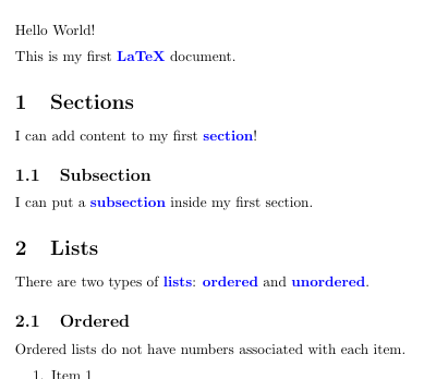
I can add content to my first \textbf{\underline{section}}!We can add this to each of our important terms in our document - maybe it looks something like this:
In a long document this would quickly become tedious. Instead, let’s
define a new command called \kw in the preamble of our
document that will do this for us:
LATEX
% The \newcommand defines a new custom command
% Highlight Keywords using the \kw{} command
\newcommand{\kw}[1]{\textbf{\underline{#1}}}
Now we can use the \kw command to highlight words in our
document:
LATEX
This is my first \kw{LaTeX} document.

\section{Sections}

I can add content to my first \kw{section}!Let’s take a minute to go through and add the \kw
command to all the keywords in our document.
- LaTeX
- section
- subsection
- lists
- ordered
- unordered
Related to the \newcommand command, we can also use the
\renewcommand command to change the definition of an
existing command. This is useful, for example, if we want to change the
effect of a command partway through a document, or if we want to change
the definition of a command that is already defined in a package. It has
an identical syntax to the \newcommand command:
Code Reuse
This also means that we can easily change the formatting of all the
words we’ve highlighted by updating the definition of the
\kw command. Let’s say we wanted to change the formatting
to bold and change the color to blue:
Let’s replace our \kw command with this new definition:
\newcommand{\kw}[1]{\textcolor{blue}{\textbf{#1}}}
When we recompile the document we should see that the formatting of our keywords has changed all at once:
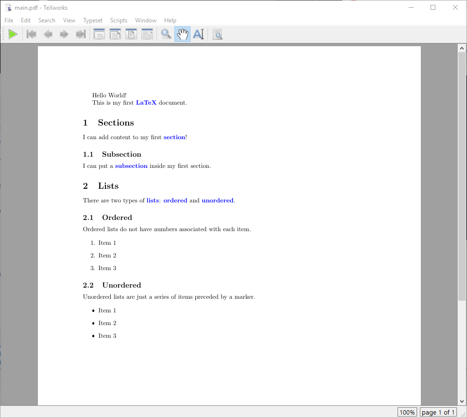
Defining Multiple Commands
We can define as many commands as we like in the preamble of our document. Let’s add another one that we can use to highlight commands in the document:
We’ll use this command in later sections.
Challenges
Challenge 1: Importing a new package
A useful package to preview what your document will look like before
your write a lot of text is the lipsum package. This
package provides sample text blocks from a common placeholder text.
How would you add the lipsum package to the preamble of your document?
Add the line \usepackage{lipsum} to the preamble of your
document.
You can then use the \lipsum command in the body of your
document to add some dummy text.
Challenge 2: What does this mean?
The definition of a new command in LaTeX is done with the
\newcommand command. The syntax for this command is:
So if we modify the \kw command we defined above to look
like this:
What would the new \kw command do? and how would we use
it?
Challenge 3: Can you write your own command with two arguments?
Suppose you want to define a new command that takes as input two words as arguments. This first word shall be written bold while the second word shall be written italic. Moreover, the first and the second word are separated by a comma followed by a whitespace.
Use \newcommand to define this command that takes two
arguments as inputs and name it \boit. Write the following
sentence into your LaTeX document using your new command
\boit:
This newly defined command highlights these two words: Apple, Banana.
The new \boit command would take two arguments: the
first argument would be used with \tetxbf{#1} to make the
first word appear bold, and the second argument would
be used with \tetxit{#2} to make the first word appear
italic. Between \tetxbf{#1} and
\tetxit{#2}, we would write , to separate both
words. We would use the new command like this:
Challenge 4: Optional arguments
New commands can be made even more flexible by defining commands that take an optional argument. Then the general LaTeX code for this looks like this:
LATEX
\newcommand{\commandname}[number of arguments][default value for the first argument]{definition}The optional argument can be accessed and changed by writing square
brackets [] directly after the \commandname in
the body of your document.
Consider the following, modified example of our \kw from
before where we now use an optional argument.
In your LaTeX file, use the new \kw command to write
down the words “Banana” in yellow, “Apple” in red, and “Blueberry” in
blue. Each word should be written in a separate line.
We can exploit the optional argument in \kw to write
down the given words very efficiently. For the first word, we change the
optional argument to “yellow”. For the second word, we stick with the
default value of “red”. For the third word, we change the optional
argument to “blue”.
- We can extend LaTeX’s functionality by adding packages to our document.
- We can define custom commands in LaTeX using the
\newcommandcommand.
After this episode, here is what our LaTeX document looks like.
Content from Fonts, Formatting and Spacing
Last updated on 2026-04-08 | Edit this page
Overview
Questions
- How can we set paragraph spacing in LaTeX?
- How can we customize text formatting in LaTeX?
- How can we align text in LaTeX?
Objectives
- Add custom spacing between paragraphs in LaTeX.
- Create a title page with custom text formatting.
Fonts
We saw earlier that we can create commands of our own in LaTeX, but
there is also a renewcommand command that let’s us change
the definition of an existing command. This might be useful if you want
the definition of a command to change throughout the document, however
there are also some commands that are pre-defined that we can modify
with this command.
For Example, we can change the font of the entire document by adding the following line to our preamble:
LATEX
% Change the font of the entire document to a monospace font
\renewcommand{\familydefault}{\ttdefault}
When you compile the document you should see that it has changed from this:
To this:
More Fonts
Unfortunately, the default LaTeX installation does not come with many
fonts. However, there are additional packages that you can include if
you are looking for a specific font. Let’s try making our document look
like it’s using the Times New Roman font. To do this, all
we need to do is add the following line to the preamble:
You can find a large selection of fonts at The LaTeX Font Catalogue, complete with examples of how to use them in your document.
When you are using lualatex (or xelatex)
for compiling you can easily use all the fonts that are installed
locally on your computer:
Paragraph Spacing
A common style in LaTeX is to have no indents for paragraphs, but to
incorporate a blank line between them. We can achieve this using the
parskip package.
We’re going to use another package here just to show off some
commands without having to write a lot of text: the lipsum
package. This package provides the \lipsum command, which
generates “Lorem Ipsum” text.
Lorem Ipsum is a common piece of placeholder text used in publishing and graphic design. It is often used to demonstrate the visual form of a document without relying on meaningful content.
The text itself comes from the first-century BC work De finibus bonorum et malorum by Marcus Tullius Cicero.
In our document, we can now use a blank line to separate paragraphs:
LATEX
\section{Formatting and Spacing}

% Generate some "Lorem Ipsum" text
% The parameters mean "include paragraphs 1 thru 2" from the "Lorem Ipsum" text
\lipsum[1-2]
Compile the document and take a look at our section. You should see that our first paragraph has no indent, and there is no blank line between it and the following paragraph. The second paragraph does have an indent. This is the default behavior in LaTeX.
Now let’s add our package:
Keep an eye on the preview pane as you compile the document. You should see that the first paragraph now has a blank line between it and the second paragraph, and there is no indent on the first line of the second paragraph.
When you use a KOMA-Script documentclass you get the same result using a global option:
Forcing a New Line
Most of the time, you should not force a new line in your document;
you almost certainly want to use a new paragraph or parskip
instead. However, there are a few places where you might want
to force a new line:
- At the end of table rows
- Inside a
centerenvironment - In poetry (the
verseenvironment)
To force a new line, we can use the \\ command.
Adding Explicit Space
We can insert a thin space (about half the normal thickness) use the
\, command.
In math mode, there are also other commands:
-
\.for a “dot” space -
\:for a “colon” space -
\;for a “thick” space -
\!for a “negative” space -
\,for a “thin” space
Very rarely, for example when creating a title page, you might want
to add explicit horizontal or vertical space. We can do this using the
\hspace and \vspace commands:
We can also use the \vfill command to fill the remaining
space on a page. This is useful for centering content vertically on a
page.
Explicit Text Formatting
We’ve touched on this in previous episodes, but we can also use the following commands to format text explicitly:
-
\textbf{}for bold text -
\textit{}for italic text -
\textrm{}for roman text -
\textsf{}for sans serif text -
\texttt{}for typewriter text -
\textsc{}for small caps text
We can set the font size in the same way. All sizes are relative to the base font size:
-
\hugefor huge text -
\largefor large text -
\normalsizefor normal text -
\smallfor small text -
\footnotesizefor footnote text
You can further customize your font size by setting the font size
explicitly with the \fontsize command. The first parameter
is the font size, and the second parameter is the “leading”, which is
the distance between the base lines of each line of text.
{\fontsize{14}{16}\selectfont \lipsum}If you want it really big:
Text Alignment
We can align text using the following commands:
-
\centeringto center text -
\raggedrightto left-align text -
\raggedleftto right-align text
Creating a Title Page
Using all of this, let’s create a simple title page for our document.
We’ll put this just after the \begin{document} command, and
enclose everything in a titlepage environment:
LATEX
\begin{titlepage}
    \centering

    \textbf{My Example Document}

    \vfill
    January 1, 2000
\end{titlepage}The titlepage environment is a special environment that
LaTeX uses to create a title page. It sets some simple formating rules,
like removing multiple columns and resetting the page number. It also
prevents styling rules we add like centering from affecting
the rest of the document.
Challenges
Challenge 1: Create a Title Page with Custom Formatting
Using the content covered, create a title page with custom formatting. Your title page should have:
- A centered title “My Custom LaTeX Title Page” in large, bold text.
- A centered subtitle in italic text, smaller than the title.
- The date centered at the bottom of the page.
You can use the commands \vspace and \vfill
to make fill blank space between the items.
Here’s an example of what your title page could look like:

Challenge 2: Adjust Paragraph Spacing
Consider the following document:
LATEX
\documentclass{article}
\usepackage{lipsum}
\begin{document}
\section{My Report}
\lipsum[1]
\lipsum[2]
\lipsum[3]
\end{document}We want our document to have no indents for paragraphs, but to have a single blank line between them. What do we need to change in the document to achieve this?
If you want to try this out, you can copy and paste the code into a
new .tex file and compile it to see the result.
We need to add the parskip package to the preamble of
our document. This will add a blank line between paragraphs and remove
the indent from the first line of each paragraph.
We also need to add a blank line between each \lipsum
command in order to create a new paragraph for each block of text.
Challenge 3: Making a custom quote block
Create a customg quote block using a center environment
and \vspace commands. See if you can make it look something
like this:

Note that there is some vertical space above and below the quote, and the text is formatted with different font sizes and styles. The quote itself is in italics, and the attribution is in small caps.
Bonus! Make a \newcommand to create a custom quote block
that you can reuse throughout your document.
Use a center environment to center the text, and use
\vspace to add space above and below the quote. Format the
text using explicit formatting options.
- Use the
parskippackage to add space between paragraphs - Force a new line with
\\ - Add explicit space with
\hspaceand\vspace - Format text explicitly with
\textbf,\textit, etc. - Align text with
\centering,\raggedright, and\raggedleft
Content from Using Graphics
Last updated on 2026-04-08 | Edit this page
Overview
Questions
- How do I include images in a LaTeX document?
Objectives
- Demonstrate how to include images in a LaTeX document.
- Show how to position images manually / automatically in a LaTeX document.
The Graphicx Package
In order to use graphics in our document, we’ll need to use the
graphicx package, which adds the
\includegraphics command to LaTeX. We’ll add this to the
preamble of our document:
We can now include several types of images in our document, including:
- JPEG
- PNG
- SVG
- EPS
Although LaTeX can handle several commonly used image formats, there
are a few which are currently incompatible with LaTeX. For example, the
webp and tiff formats. If you have an image in
one of these formats, you will need to convert it to a compatible format
before including it in your document.
For the purposes of this lesson, we’ll use the following image:

Download this image to your computer either be right-clicking on the image and selecting “Save Image As…” or by clicking on the image and saving it from the browser.
You can use any image you like for this lesson. Just make sure to
replace my-awesome-image.png with the name of your image in
the following examples.
Place the image in the same directory as your LaTeX document so that LaTeX can find it when we compile the document.
There is a command called \graphicspath that allows you
to specify a directory where LaTeX should look for images. This can be
useful if you have a dedicated folder for your images. For example, if
you have a folder called images in the same directory as
your LaTeX document, you can add the following line to your
preamble:
This tells LaTeX to look for images in the images folder
when you use the \includegraphics command.
Including an Image in a LaTeX Document
Now that we have our image, we can include it in our document using
the \includegraphics command:
LATEX
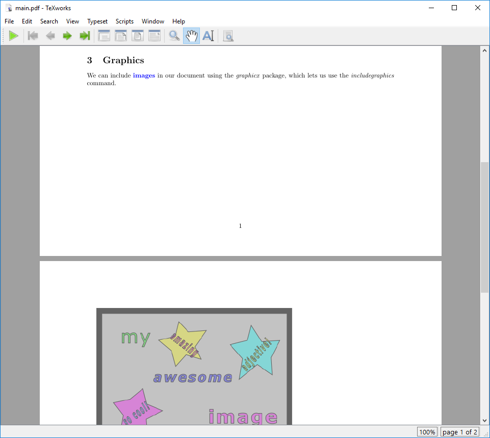
\section{Graphics}
We can include \kw{images} in our document using the \cmd{graphicx} package, which lets us use the
\cmd{includegraphics} command.
\includegraphics{my-awesome-image}Your document should now look like this:
If you just want to see how an image might look in your document
without having to find one, you can use the filepath
example-image in the \includegraphics command.
This will display a placeholder image in your document that you can
replace later.
Adjusting the appearance of the image
But wait! The image is too big, and it doesn’t fit on the page, so LaTeX has moved it to the next page. Since the image is a little too large to fit on the same page as the text, LaTeX has moved it automatically to the next page. Let’s address that by making the image smaller.
We can adjust the appearance of the image by passing options to the
\includegraphics command, just like we did earlier with the
geometry package. For example, we can specify the height of
the image:
LATEX
\subsection{Small Image}
We can pass parameters to the \cmd{includegraphics} command to adjust the appearance of the image.
\includegraphics[height=2cm]{my-awesome-image}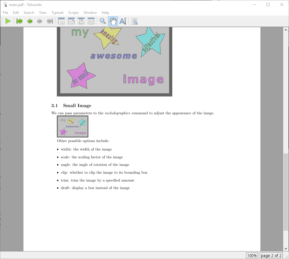
Some other possible options from the graphicx package
include:
-
width: the width of the image -
scale: the scaling factor of the image -
angle: the angle of rotation of the image -
clip: whether to clip the image to its bounding box -
trim: trim the image by a specified amount -
draft: display a box instead of the image
The \linewidth command can be used to specify the width
of the image relative to the width of the text. For example,
width=0.5\linewidth would make the image half the width of
the text, rather than having to specify exact values.
This is particuarly useful in multi-column layouts, where the width of the text may vary depending on the number of columns.
Overfull Boxes
Now that we have included an image in our document, we have another kind of error we might encounter - “overfull boxes”. This happens when the content of a box (like an image or a paragraph of text) is too large to fit within the specified dimensions of the box, and it overflows into the margins.
The following code generates this warning message:
LATEX
\documentclass{article}
\usepackage{graphicx}
\begin{document}
\section{Adding a rotated image}
We can rotate an image by setting the "angle" parameter:
\includegraphics[scale=2, angle=45]{example-image}
\end{document}The document compiles successfully, but there was some text that briefly appeared in the console output. Let’s look at the .log file to see what it says:
Overfull \hbox (390.7431pt too wide) in paragraph at lines 10--11
[][]
[]
[1
{c:/texlive/2025/texmf-var/fonts/map/pdftex/updmap/pdftex.map}]
Overfull \vbox (170.7431pt too high) has occurred while \output is active []
[2 <./example-image.png>] (./main.aux)This means that the text or image is too wide or too tall for the page, and it is overflowing into the margins. To fix this, we can adjust the size of the image or the layout of the page to ensure that everything fits within the specified dimensions.
Note that there may be times when we actually want the image to overflow into the margins, for example if we want to include an image that extends to the edges of the page. In this case, we can ignore the warning message and proceed with our document - this warning will not prevent our document from compiling successfully.
Positioning the image
We can place the image inside of an environment to help position it
in the document. Let’s try placing the \includegraphics
command inside of a \begin{center} and
\end{center} environment:
LATEX
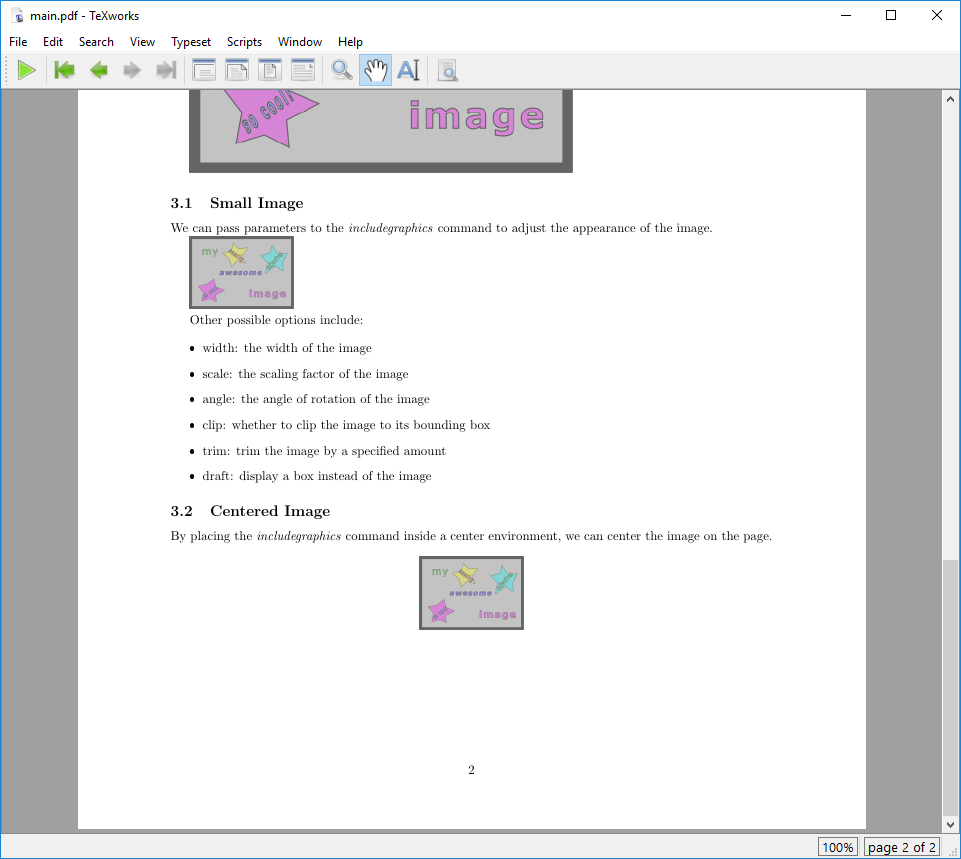
\subsection{Centered Image}
By placing the \cmd{includegraphics} command inside a center environment, we can center the
image on the page.
\begin{center}
\includegraphics[height=2cm]{my-awesome-image}
\end{center}You should see that the image is now centered on the page:
“Floating” Images
It’s often the case that images need to “float” around the document as new text is added or removed. this is called a “floating” image. Images are normally included as floats so that we don’t end up with large gaps in the document.
To make an image float, we can use the figure
environment:
LATEX
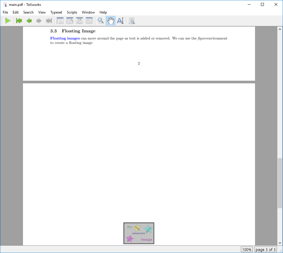
\subsection{Floating Image}
\kw{Floating images} can move around the page as text is added or removed. We can use the
\cmd{figure}environment to create a floating image.
\begin{figure}
\centering
\includegraphics[height=2cm]{my-awesome-image}
\end{figure}When we render the document, we can see that, even though we placed the image at the end of the document, it appears at the top of the page:
You might have noticed that instead of using the
\begin{center} and \end{center} environment,
we used the \centering command inside of the
figure environment. This is because the figure
environment is a floating environment, and the \centering
command is the recommended way to center content inside of a floating
environment.
Controlling the Position of a Floating Image
We can pass parameters to the figure environment to
control the position of the floating image:
-
h: Place the float “here” (where it appears in the code) -
t: Place the float at the “top” of the page -
b: Place the float at the “bottom” of the page -
p: Place the float on a “page” by itself
It is also possible to combine these options. For example, to place
the float here if possible, but otherwise at the top of the page, we can
use the ht option. Let’s update our figure
environment to use the ht option:
LATEX
\begin{figure}[ht]
\centering
\includegraphics[height=2cm]{my-awesome-image}
\end{figure}
Control the position of a floating image by passing parameters to the \cmd{figure} environment:
\begin{itemize}
\item h: "here"
\item t: "top"
\item b: "bottom"
\item p: "page"
\end{itemize}You can use the package wrapfig together with
graphicx in your preamble. This makes the
wrapfigure environment available and we can place an
\includegraphics command inside it to create a figure
around which text will be wrapped. Here is how we can specify a
wrapfigure environment:
We will describe the wrapfigure environment in more
detail in one of the challenges below.
Adding a Caption
We can add a caption to our image by using the \caption
command inside of the figure environment:
LATEX
\subsection{Caption}
We can add a \kw{caption} to our floating image by using the \cmd{caption} command inside of the
\cmd{figure} environment.
\begin{figure}
\centering
\includegraphics[height=2cm]{my-awesome-image}
\caption{This is a caption for our image.}
\end{figure}When we render the document, we can see that the caption appears below the image:
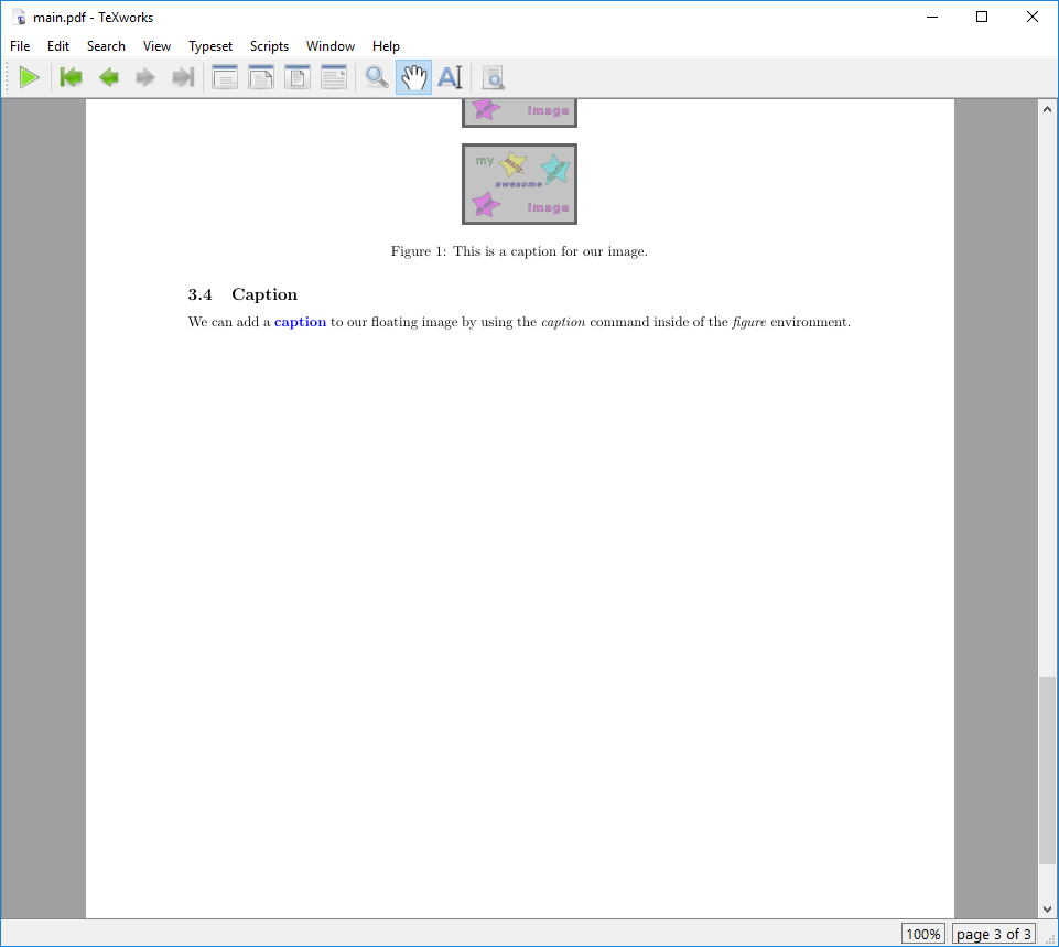
Note that the caption is automatically numbered “Figure 1”. Very handy! We’ll see how we can automatically reference figures and tables in a later episode.
Another package that we can use to work with images in LaTeX is the
hvfloat package. This package is an alterantive way of
controlling the position of floating elements in LaTeX, like images and
tables. It provides a more flexible way of positioning floats allowing
us to, for example, place a float at the bottom of the page, even if
there is not enough space for it to fit.
There’s a command called \listoffigures that will
generate a list of all of the figures in your document. This will only
list the figures that have a caption, so make sure to add a caption to
any figure you want to be included in the list.
Challenges
Challenge 1: Can you do it?
Consider again our running example of example-image.PNG.
Include this image into your LaTeX document by using the
figure environment. Make sure that your image is centered
and rotate the image by 45 degree. Add the following caption to your
image: “This caption has a bold word included.” How
would your LaTeX look like?
We use the \centering command in the figure
environment and specify angle=45 to rotate the image.
Challenge 2: What is wrong here?
Have a look at the following LaTeX code:
LATEX
\documentclass{article}
\begin{document}
\centering
\begin{figure}
\includegraphics[height=3cm, draft]{my-awesome-image}
\caption{This caption has a \textbf{bold} word included.}
\end{figure}
\end{document}Can you spot all the errors in this LaTeX code? Change the code such that the image is displayed with a height of 3cm, width of 4cm and centered.
- the command
\usepackage{graphicx}is missing in the preamble. - the
\centeringcommand has to be placed into thefigureenvironment. - the
draftargument has to be removed from the\includegraphicscommand andwidth=4cmadded.
The corrected LaTeX code looks like this:
Challenge 3: Making a command for images
In the previous section, we created a command to highlight keywords
in our document. Let’s create a new command to make it easier to include
images in our document. We’ll create a command called
\centeredimage that takes two arguments: the image filename
and the caption. The resulting image should be centered on the page and
have a caption below it. Use the example-image.png from earlier in this
episode.
Your file should look like this:
LATEX
\documentclass{article}
\usepackage{graphicx}
% Define our new command
%%% YOUR COMMAND HERE %%%
\begin{document}
\centeredimage{example-image.png}{"My Image"}
\centeredimage{example-image.png}{"My Other Image"}
\end{document}And your output should look like this.
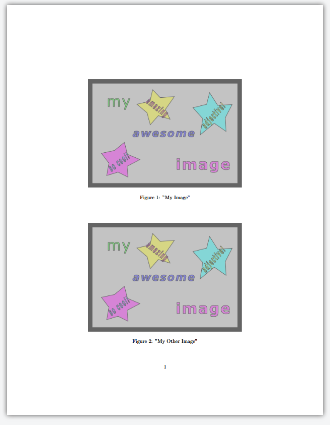
Reminder: The syntax for creating a new command is:
LATEX
\documentclass{article}
\usepackage{graphicx}
% Define our new command
\newcommand{\centeredimage}[2]{
\begin{figure}
\centering
\includegraphics{#1}
\caption{#2}
\end{figure}
}
\begin{document}
\centeredimage{my-awesome-image}{"My Image"}
\centeredimage{my-awesome-image}{"My Other Image"}
\end{document}Challenge 4: The wrapfig
package.
Have a look at the following LaTeX code that uses the
wrapfigure environment. Can you already guess how the
images will be displayed in your document?
LATEX
\documentclass{article}
\usepackage{wrapfig}
\usepackage{graphicx}
\begin{document}
\begin{wrapfigure}{r}{0.1\textwidth}
\centering
\includegraphics[width=0.1\textwidth, height=0.1\textwidth]{my-awesome-image}
\end{wrapfigure}
The package wrapfigure lets you position images around your text.
That comes in handy if you want to integrate images seamlessly into your written sentences.
Therefore, I add a few more sentences here to showcase this integration to you.
\begin{wrapfigure}{l}{0.1\textwidth}
\centering
\includegraphics[width=0.1\textwidth, height=0.1\textwidth]{example-image.PNG}
\end{wrapfigure}
Be careful, you need both packages, wrapfig and graphicx, in your preamble to display your images
and wrap them accordingly. There are several ways to display images, depending on the arguments you
specify. For instance, you can scale the image width according to the width of the text.
\end{document}The first image will be placed at the right of the following
paragraph of text as {r} is specified as an argument within
the first wrapfigure environment. The second image will be
placed at the left of its following paragraph of text as
{l} is specified as an argument within the second
wrapfigure environment. Moreover, both images are scaled by
being 0.1 of the width of the text in your document.
- The
graphicxpackage allows us to include images in our LaTeX document. - We can adjust the appearance of images using options in the
\includegraphicscommand. - We can position images manually or automatically using environments
like
centerandfigure. - Floating images can move around the page as text is added or removed.
- We can control the position of floating images using parameters in
the
figureenvironment. - We can add captions to floating images using the
\captioncommand.
After this episode, here is what our LaTeX document looks like.
Content from Tables
Last updated on 2026-04-08 | Edit this page
Overview
Questions
- How do I add tables to a LaTeX document?
- How can I format a table in a LaTeX document?
Objectives
- Create a table in a LaTeX document.
- Customize the appearance of a table in a LaTeX document.
- Add horizontal lines to a table in a LaTeX document.
Defining Tables
Tables in LaTeX are set using the tabular environment.
For our purposes here, we are going to use the array
package to create a table, which provides additional functionality for
creating tables. We’ll add this to the preamble of our document:
As we start to add more and more packages to our preamble, it can get a bit unwieldy. For now, let’s just keep them alphabetized to make it keep things organized. Our imports should now look like this:
In order to create a table, we need to tell latex how many columns we will need and how they should be aligned.
Available column types are:
| Column Type | Description |
|---|---|
l |
left-aligned |
c |
centered |
r |
right-aligned |
p{width} |
a column with fixed width; the text will be automatically line wrapped and fully justified |
m{width} |
like p, but vertically centered compared to the rest of the row |
b{width} |
like p, but bottom aligned |
w{align}{width} |
prints the contents with a fixed width, silently overprinting if things get larger. (You can choose the horizontal alignment using l, c, or r.) |
W{align}{width} |
like w, but this will issue an overfull box warning if things get too wide. |
The columns l, c and r will have the natural width of the widest
entry in the column. Each column must be declared, so if you want a
table with three centered columns, you would use ccc as the
column declaration.
Creating a Table
Now that we have the array package loaded and we know how to define
columns, we can create a table using the tabular
environment.
Note that the & and \\ characters are
aligned in our example. This isn’t strictly necessary in LaTeX, but it
makes the code much easier to read.
LATEX
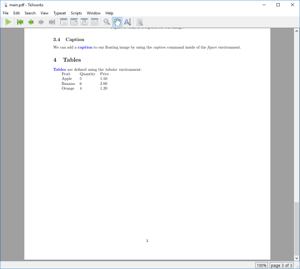
\section{Tables}
\kw{Tables} are defined using the \cmd{tabular} environment.
\begin{tabular}{lll}
Fruit & Quantity & Price \\
Apple & 5 & 1.50 \\
Banana & 6 & 2.00 \\
Orange & 4 & 1.20 \\
\end{tabular}This will create a table with three columns, all left-aligned. The
values of each row are separated by & and the rows are
separated by \\. We do not yet have any horizontal lines in
the table, so it will look like this:
If your table has many columns, it may get cumbersome to write out
the column definitions every time. In this case you can make things
easier by using *{num}{string} to repeat the string
num times. For example, in our table above, we can instead
write:
Adding Horizontal Lines
We’re going to introduce another package here: booktabs.
This package provides a few commands that make it easier to create
professional looking tables. To use it, add the following to your
preamble:
booktabs provides three commands for creating horizontal
lines in your table:
-
\toprule: creates a line at the top of the table -
\midrule: creates a line in the middle of the table -
\bottomrule: creates a line at the bottom of the table
Horizontal lines make tables easier to read and understand, and they can be used to separate the header from the body of the table, and the body from the footer. We can insert these commands into our table to add horizontal lines:
LATEX
\subsection{Tables with Horizontal Lines}
We can use the \cmd{\textbackslash toprule}, \cmd{\textbackslash midrule}, and
\cmd{\textbackslash bottomrule} commands from the \cmd{booktabs} package to create horizontal
lines in our table.
\begin{tabular}{*{3}{l}}
\toprule
Fruit & Quantity & Price \\
\midrule
Apple & 5 & 1.50 \\
Banana & 6 & 2.00 \\
Orange & 4 & 1.20 \\
\bottomrule
\end{tabular}Your table should look something like this:
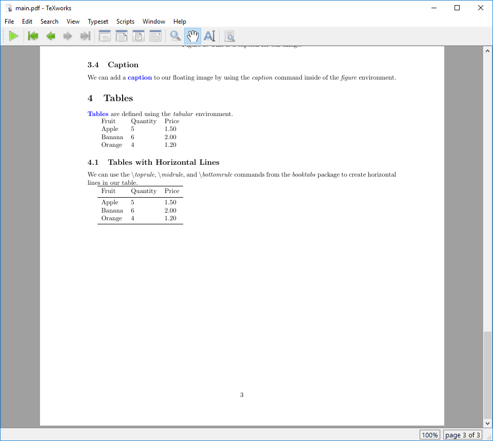
A general recommendation is to use lines sparsely in your tables, and vertical lines should be avoided.
Partial Horizontal Lines
Another useful feature of booktabs is the ability to
create partial horizontal lines with the \cmidrule command.
This command accepts the arguments {number-number}, where the first
number is the column to start the line and the second number is the
column to end the line.
LATEX
\subsection{Partial Horizontal Lines}
The \cmd{\textbackslash cmidrule} command can be used to create partial horizontal lines in a
table. The command accepts the arguments {number-number}, where the first number is the column to
start the line and last number is the column to end the line.
\begin{tabular}{*{3}{l}}
\toprule
Fruit & Quantity & Price \\
\midrule
Apple & 5 & 1.50 \\
Banana & 6 & 2.00 \\
Orange & 4 & 1.20 \\
\cmidrule{3-3}
Total & 15 & 28.20 \\
\bottomrule
\end{tabular}This table should come out looking something like this:
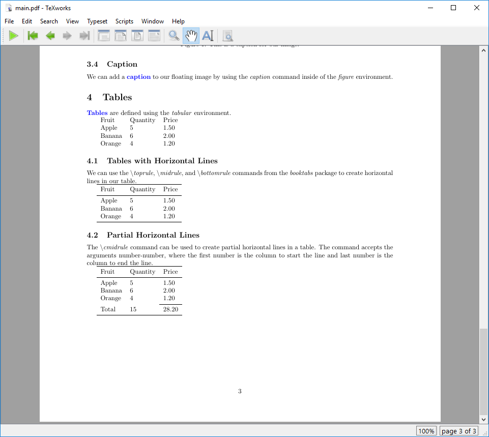
Merging Cells
We can merge cells horizontally using the \multicolumn
command. This command takes three arguments:
- The number of cells which should be merged
- The alignment of the merged cell (l, c, or r)
- The contents of the merged cell
LATEX
\subsection{Merging Cells}
Merge cells horizontally using the \cmd{\textbackslash multicolumn} command. This command takes
three arguments:
\begin{itemize}
\item The number of cells which should be merged
\item The alignment of the merged cell (l, c, or r)
\item The contents of the merged cell
\end{itemize}
\begin{tabular}{*{3}{l}}
\toprule
\multicolumn{3}{c}{Overall Inventory} \\
Fruit & Quantity & Price \\
\midrule
Apple & 5 & 1.50 \\
Banana & 6 & 2.00 \\
Orange & 4 & 1.20 \\
\midrule
\multicolumn{2}{c}{Summary} \\
Total & 15 & 28.20 \\
\bottomrule
\end{tabular}Vertical merging is supported in LaTeX by using the
multirow package which has the \multirow
command equipped with it. It is similarly structured as
\multicolumn by using three arguments:
- The number of rows which should be merged
- The width of the column (i.e. 4em)
- The contents of the merged rows.
You can find an example in the challenges below.
This will create a table that looks like this:
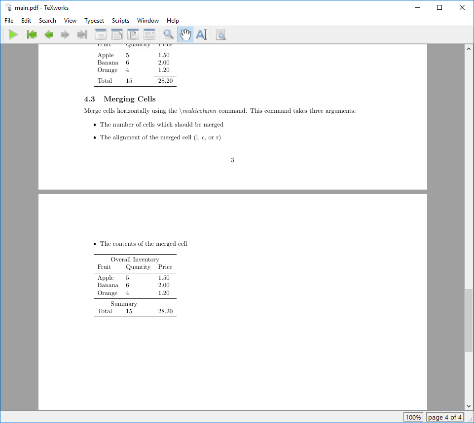
Positioning Tables
By default, tables will be placed exactly where they are defined in
the LaTeX document. We saw in the earlier section on graphics that we
can use the figure environment to create floating figures,
which gives us a lot of flexability where exactly the figure will be
placed in the document.
We can do the same thing with tables by using the table
environment. This will allow us to use the same placement specifiers
that we used for figures (h, t, b, p, and !). We can also add a caption
to our table using the \caption command:
Challenges
Challenge 1: Can you do it?
Try to replicate the following table in LaTeX:
| Make | Model | Sold |
|---|---|---|
| Volkswagen | Golf | 7,687 |
| Skoda | Octavia | 4,078 |
| Seat | Leon | 3,922 |
| Volkswagen | Passat | 3,776 |
| Mercedes | GLK,GLC | 3,143 |
| Total | 22,606 |
Your LaTeX version should look something like this:
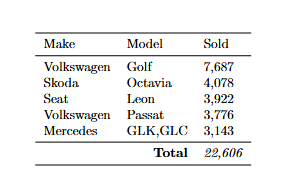
Note that the last row is a bit different from the others. The first two columns re merged, the text “Total” is right-aligned and bold, and the value in the last column is italicized.
(Data for this challenge is from Statista)
Here’s some code to get you started:
LATEX
\begin{tabular}{Something goes here...}
Something goes here...
Make & Model & Sold \\
Something goes here...
Volkswagen & Golf & 7,687 \\
Skoda & Octavia & 4,078 \\
Seat & Leon & 3,922 \\
Volkswagen & Passat & 3,776 \\
Mercedes & GLK,GLC & 3,143 \\
Something goes here...
How do we get the only two cells here? And then they need to be right-aligned and bolded...
Something goes here...
\end{tabular}For the last row, we need to merge the first two cells together. We
can do this using the \multicolumn command. If we then
merge these two cells, then right aligning the text…
LATEX
\documentclass{article}
\usepackage{array}
\usepackage{booktabs}
\begin{document}
\begin{tabular}{lll}
\toprule
Make & Model & Sold \\
\midrule
Volkswagen & Golf & 7,687 \\
Skoda & Octavia & 4,078 \\
Seat & Leon & 3,922 \\
Volkswagen & Passat & 3,776 \\
Mercedes & GLK,GLC & 3,143 \\
\midrule
\multicolumn{2}{r}{\textbf{Total}} & \textit{22,606} \\
\bottomrule
\end{tabular}
\end{document}Challenge 2: Merging rows.
Consider the following LaTeX code that creates a table using the
command \multirow. Can you guess how this table will look
like? How many columns will it have? How many rows? Are any rows or
columns combined?
LATEX
\documentclass{article}
\usepackage{booktabs}
\usepackage{multirow}
\begin{document}
\begin{tabular}{*{4}{l}}
\toprule
& Food & Quantity & Price \\
\midrule
\multirow{3}{4em}{Fruit} & Apple & 5 & 1.50 \\
& Banana & 6 & 2.00 \\
& Orange & 4 & 1.20 \\
\midrule
\multirow{2}{4em}{Cheese} & Brie & 2 & 3.30 \\
& Asiago & 3 & 2.90 \\
\bottomrule
\end{tabular}
\end{document}The multirow command is used here to merge rows
together. In the case here, we have two multirow commands,
one for the “Fruit” category and one for the “Cheese” category. The
first argument of the multirow command specifies how many
rows should be merged together, the second argument specifies the width
of the merged cell, and the third argument specifies the contents of the
merged cell.
The table created by this code will look like this:
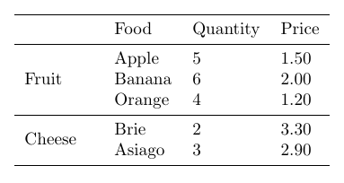
Challenge 3: Adding merged rows to your table.
Consider again the LaTeX code for the table in challenge 2. Add four more rows to this table that contain information about the following four sorts of bread:
- Brioche, 3, 3.00
- Bagel, 2, 3.50
- Matzah, 4, 3.60
- Naan, 2, 3.40
Use \multirow to subsume those bread types under the
category “Bread”.
LATEX
\documentclass{article}
\usepackage{booktabs}
\usepackage{multirow}
\begin{document}
\begin{tabular}{*{4}{l}}
\toprule
& Food & Quantity & Price \\
\midrule
\multirow{3}{4em}{Fruit} & Apple & 5 & 1.50 \\
& Banana & 6 & 2.00 \\
& Orange & 4 & 1.20 \\
\midrule
\multirow{2}{4em}{Cheese} & Brie & 2 & 3.30 \\
& Asiago & 3 & 2.90 \\
\midrule
\multirow{4}{4em}{Bread} & Brioche & 3 & 3.00 \\
& Bagel & 2 & 3.50 \\
& Matzah & 4 & 3.60 \\
& Naan & 2 & 3.40 \\
\bottomrule
\end{tabular}
\end{document}Challenge 4: Making the Table Colorful
We used the xcolor package to add color to our text in
an earlier episode. Can you use the xcolor package to make
the header and summary rows of the table in Challenge 1 a different
color? What about changing the color of the text in the summary row? Can
we make the rows of the table alternate colors?
A few things that will help you:
- We need to import the
xcolorpackage in the preamble of our document. - The
xcolorpackage doesn’t automatically support coloring tables, so we need to add thetableoption to the package import. \rowcolor{(<color>}\rowcolors{<starting row number>}{<color1>}{<color2>}- You can make lighter versions of colors by adding
!<percentage>to the color name. For example,red!10is a light red color, whilered!90is a darker red color.
There’s no right answer to this challenge, so feel free to experiment with different colors!
Here’s an example of what you can do:
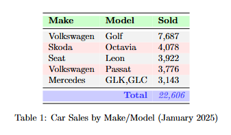
LATEX
\documentclass{article}
\usepackage{array}
\usepackage{booktabs}
\usepackage[table]{xcolor} % Import xcolor with the table option
\begin{document}
\begin{table}[ht]
\centering
\rowcolors{2}{red!10}{gray!10} % Alternate row colors between red and gray
\begin{tabular}{lll}
\toprule
\rowcolor{green!20} % Set the header row color to green
Make & Model & Sold \\
\midrule
Volkswagen & Golf & 7,687 \\
Skoda & Octavia & 4,078 \\
Seat & Leon & 3,922 \\
Volkswagen & Passat & 3,776 \\
Mercedes & GLK,GLC & 3,143 \\
\midrule
\rowcolor{blue!20} % Set the summary row color to blue
\multicolumn{2}{r}{
% Set the text color to blue and bold for the summary row
\textbf{\textcolor{blue!75}{Total}}} & \textit{\textcolor{blue!75}{22,606}} \\
\bottomrule
\end{tabular}
\caption{Car Sales by Make/Model (January 2025)} % Add a caption to the table
\end{table}
\end{document}- Tables in LaTeX are created using the
tabularenvironment. - The
arraypackage provides additional functionality for creating tables. - The
booktabspackage provides commands for creating horizontal lines in tables. - The
\multicolumncommand can be used to merge cells in a table. - The
\multirowcommand in themultirowpackage can be used to merge rows in a table.
After this episode, here is what our LaTeX document looks like.
Content from Adding Cross References
Last updated on 2026-04-10 | Edit this page
Overview
Questions
- How can I ensure that numbers in my document are automatically updated?
- How can I refer to numbered elements in my document?
Objectives
- Insert a cross-reference in a LaTeX document.
- Refer to a cross-referenced element in a LaTeX document.
Cross References
When writing a document of any length, you’ll often want to refer to numbered elements such as figures, tables, equations, or sections. LaTeX provides a way to automatically number these elements and refer to them in your text.
Label and Ref
To have LaTex remember a specific spot in your document, you have to
use the \label{} command to mark it, and the
\ref{} command to refer to it. For example:
LATEX
\section{Cross References}
\label{sec:cross-references}
\subsection{Material for the Introduction}
In this section, we introduce two new concepts:
\begin{table}
\begin{tabular}{cp{9cm}}
\toprule
Command & Description \\
\midrule
\kw{label} & Marks a spot in the document \\
\kw{ref} & Refers to a marked spot in the document \\
\bottomrule
\end{tabular}
\caption{Main commands for referencing in \LaTeX.}
\label{tab:cross-reference-commands}
\end{table}
We can \kw{refer} to the section with the \cmd{ref} command, like this: \ref{sec:cross-references}.
We can likewise refer to the table like this: \ref{tab:cross-reference-commands}.The sec and tab prefixes in the
\label{} command are not required, but they help to
identify the type of element being labeled. This is especially useful
when you have many labels in your document.
When you hit compile, you may notice that the \ref{}
command does not return the correct references and instead shows
question marks (??). This is because LaTeX needs to compile the document
twice. Once to gather all the labels and references, and a second time
to resolve them. If you see question marks, just compile the document
again, and it should work correctly.
The label command always refers to the previous numbered entry: a
section, a table, a figure, etc. This means that the
\label{} command should always come after the
numbered element you want to refer to.
Note that the ref command does not insert the section or
table name, but rather the number associated with it. We would still
write “Refer to Table \ref{tab:cross-reference-commands}”, but the
benefit is that if the table number changes because we’ve added or
removed sections before it, the reference will update automatically.
There are packages that can provide more advanced cross-referencing
capabilities, such as the cleveref package, which can
automatically detect the type of element being referenced and insert the
appropriate name. For more details about this, refer to the references
section.
cleveref allows the format of cross-references to be
formatted automatically, so that the “type” of the referenced element
(e.g., figure, table, section) is included in the reference text. The
\cref command is used to create these references.
If you want the references to be clickable in the PDF, you can use
the hyperref package:
This package automatically makes all references clickable, allowing you to jump to the referenced element in the PDF document. However be aware that this can sometimes cause issues with other packages, so it’s best to load it last in your preamble.
Note that in order to avoid compilation issues, the
hyperref package should be loaded after all other packages
in your preamble, except for packages that are specifically designed to
work with hyperref, like cleveref.
Challenges
Challenge 1: Add a figure, then reference it.
In your LaTeX document, include the image
example-image.PNG and cross-reference it in the text. Make
sure the figure has a caption and is labeled and centered properly. Use
the \includegraphics command to add the image and wrap it
in a figure environment. Then, refer to it in the text
using the \ref command.
You may find the following LaTeX template helpful.
LATEX
\documentclass{article}
\usepackage{graphicx}
\begin{document}
\section{Cross-referencing Figures}
Here is an example of a figure in the document. We will refer to it later in the text.
% Figure goes here
In the text, we can refer to the figure using its label: % Something goes here
\end{document}The goal will be to have something that looks like this:
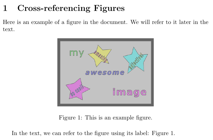
Use the figure environment to wrap the image, and use
the \includegraphics command to add the image. In order to
center the image, you can use the \centering command inside
the figure environment.
Make sure that the \label{} command comes after the
\caption{} command, and that the \ref{}
command refers to the correct label.
LATEX
\documentclass{article}
\usepackage{graphicx}
\begin{document}
\section{Cross-referencing Figures}
Here is an example of a figure in the document. We will refer to it later in the text.
\begin{figure}[ht]
\centering
\includegraphics[height=4cm]{example-image.PNG}
\caption{This is an example figure.}
\label{fig:example-image}
\end{figure}
In the text, we can refer to the figure using its label: Figure \ref{fig:example-image}.
\end{document}Challenge 2: Where does the reference go?
We mentioned that the \label{} command should always
come after the numbered element you want to refer to. What do you think
would happen if we put the \label{} command before the
numbered element? For example:
LATEX
\documentclass{article}
\usepackage{lipsum}
\begin{document}
\section{Introduction}
\label{sec:intro}
\lipsum[1]
\label{sec:methods}
\section{Methodology}
\lipsum[2]
\section{Findings}
As indicated in Section \ref{sec:methods}, \lipsum[3][2]
\end{document}The \lipsum package is a nice way of quickly
generating large amounts of placeholder text - great if you just want to
get an idea of how your document will look!
Before you run the code, think about what will happen. What do you expect the output to be? Run the code and see if your expectations were correct. Why or why not?
You might have expected the output to be either “As indicated in
Section 2, …” or “As indicated in Section ???”, but it actually returns
“As indicated in Section 1, …”. This is because the
\label{} command marks the section number
immediately preceding it. In this case, the
\label{} command is placed before the
\section{Methodology} command, so it marks the section
number of the previous section, which is the Introduction
section. The fact that the Introduction section already has
a label does not matter.
Challenge 3a: What’s wrong with this code?
Here’s a section from a larger document. Why might the references not be working as expected? (This is a tiny but common issue!)
LATEX
\section{Findings}
\label{sec:findings}
\begin{table}[ht]
\centering
\begin{tabular}{lll}
\toprule
Color & Pre-treatment & Post-treatment \\
\midrule
Blue & 30\% & 35\% \\
Green & 15\% & 55\% \\
Red & 10\% & 12\% \\
\bottomrule
\end{tabular}
\caption{Findings from the survey.}
\label{tab:findings}
\end{table}
As shown in \ref{tab:findings} post-treatment values are higher...The document compiles without error, but the reference text has an issue. What is it? Why does this happen?
The \ref{} command is correctly written, but the
\ref{} command only returns the number of the label it is
referring to. In this case, it will return the number of the table, not
the name of the table. To fix this, you can write “As shown in Table
\ref{tab:findings}…”
Challenge 3b: Make it easier with !
In the previous challenge, we had to write “As shown in Table
\ref{tab:findings}…” to get the correct reference text. This is because
the \ref{} command only returns the number of the label it
is referring to, and does not include the type of element (e.g., table,
figure, section).
cleverref is a package that can automatically detect the
type of element being referenced and insert the appropriate name. Try to
update this example to use the cleverref package and the
\cref{} command to make the reference text more
automatic.
LATEX
\documentclass{article}
\usepackage{booktabs}
\usepackage{cleveref}
\begin{document}
\section{Findings}
\label{sec:findings}
\begin{table}[ht]
\centering
\begin{tabular}{lll}
\toprule
Color & Pre-treatment & Post-treatment \\
\midrule
Blue & 30\% & 35\% \\
Green & 15\% & 55\% \\
Red & 10\% & 12\% \\
\bottomrule
\end{tabular}
\caption{Findings from the survey.}
\label{tab:findings}
\end{table}
As shown in \cref{tab:findings} post-treatment values are higher...
\end{document}- The
\label{}command marks a spot in the document. - The
\ref{}command refers to a marked spot in the document.
After this episode, here is what our LaTeX document looks like.
Content from Mathematics
Last updated on 2026-04-08 | Edit this page
Overview
Questions
- How do I add mathematical expressions to a LaTeX document?
Objectives
- Create Inline and Display Math Mode expressions in LaTeX
Math Mode
Typesetting mathematical expressions in LaTeX is one of its greatest strengths. We can mark up mathematical content in a logical way in what is known as math mode.
There are two kinds of math mode in LaTeX:
- Inline math mode: for typesetting math within a line of text
- Display math mode: for typesetting math on its own line
AMS Math Package
We can use the base LaTeX math mode commands to create mathematical
expressions, but in practice, the amsmath package is
frequently used, as it provides several additional features and
environments for typesetting complex mathematical expressions.
We will add the amsmath package to our document in the
preamble:
Inline Math Mode
Inline math mode is marked using a pair of dollar sign symbols
($ ... $). It is also possible to use the notation
\(...\) to mark inline math mode. Simple expressions are
entered without any special markup, and you’ll see that the math is
spaced out nicely and has letters in italic.
LATEX
\section{Mathematics}
There are two kinds of math mode in LaTeX: inline and display. Inline math mode is marked with
a pair of dollar signs, whereas display math mode is marked with a pair of square brackets.
\subsection{Inline Math Mode}
The Pythagorean theorem is $a^2 + b^2 = c^2$.There are a lot of symbols and specialist math mode commands available in LaTeX:
- Superscripts:
x^2 - Subscripts:
x_1 - Greek letters:
\alpha,\beta,\gamma, etc. - Operators:
\times,\div,\sin,\log, etc. - Fractions:
\frac{numerator}{denominator} - Roots:
\sqrt{expression} - Sums and integrals:
\sum,\int,\oint, etc. - Brackets:
(),[],{},\langle,\rangle, etc.
You can also enter inline math mode using the \(...\)
notation, which is equivalent to using the dollar sign notation.
Display Math Mode
Display math mode uses the exact same commands as inline math mode,
but it is centered by default and is intended for larger equations that
are “part of a paragraph”. It is also started and ended with a pair of
square brackets (\[ ... \]).
Remember that [ and ] are special
characters in LaTeX, which is why we have to “escape” it with a
backslash(\) here.
Math Mode in LaTeX is not just for LaTeX users! It is also used other tools like Jupyter Notebooks, R Markdown and many markdown processors. There are even extensions for Google Docs and Microsoft Word that allow you to use LaTeX math mode.
Math in Enviroments
We can include math in an environment called equation to
number the equations:
LATEX
\subsection{Math in Environments}
The quadratic formula is:
\begin{equation}
x = \frac{-b \pm \sqrt{b^2 - 4ac}}{2a}
\label{eq:quadratic}
\end{equation}
This will allow us to refer to the equation later in the document with \cmd{ref} like this:
Refer to Equation \ref{eq:quadratic}.We can now refer to this equation using the \ref
command, just like we did in the previous section:
amsmath Options
Mathematical notation is very rich, and the tools in the LaTeX kernel
are sometimes not enough to cover everything. The amsmath
package extends the capabilities of LaTeX for more complex mathematical
typesetting. Let’s try it out:
Add the following to your document:
(In the preamble)
(In the body)
That look ok, but we really want the equations to be aligned
vertically, not centered on the page. We can use the align
environment from the amsmath package to do this:
LATEX
\subsection{The `amsmath` Package}
Solve the following recurrence for $ n,k\geq 0 $:
\begin{align*}
Q_{n,0} &= 1 \quad Q_{0,k} = [k=0]; \\
Q_{n,k} &= Q_{n-1,k}+Q_{n-1,k-1}+\binom{n}{k}, \quad\text{for $n$, $k>0$.}
\end{align*}The align* environment makes the equations line up on
the amperstand (&)
There’s far too many options to cover here, but the
amsmath User Guide contains many more examples.
Challenges
Challenge 1: Can you do it?
See if you can write the following mathematical expression in LaTeX:
- Special Relativity: t’ = t / sqrt(1 - v^2 / c^2)
Challenge 3: The amsmath package
and referencing equations
Add the following equation to your document: E = mc^2. For this, use
the amsmath package and a numbered align
environment. Label the equation using \label. Then, use the
\ref command to refer to the equation in the text. You may
find the following LaTeX template helpful:
LATEX
\documentclass{article}
\usepackage{amsmath} % For better equation formatting
\begin{document}
\section{Referencing Equations}
We can include a numbered equation as follows:
\begin{equation}
E = mc^2
\label{eq:energy}
\end{equation}
Now, we refer to the equation in the text. The famous equation is \ref{eq:energy}.
\end{document}Scientific Units
To write numbers with their scientific unit you can use the package
\siunitx. This provides various commands, so that instead
of writing
you write
You load the package in your preamble
Using the specifically provided macros of the package has several benefits.
Consistent formatting All numbers and units are printed with the correct spacing and font shape.
Locale and digit grouping You can automatically switch decimal markers (comma vs. point, depending on your current language/locale of the section) and group digits:
LATEX
\num{12345.678} % prints “12 345.678” or “12 345,678” depending on locale
\numlist{11;33;55;77}
\numproduct{11 x 33}
\numrange{11}{33}- Unit parsing Composite units are built from predefined macros:
LATEX
\qty{9.81}{\metre\per\second\squared}
\qty{1}{\kilo\gram\metre\per\second\squared}
\qty[per-mode = symbol]{1}{\kilo\gram\metre\per\second\squared}-
Uncertainties, lists and ranges Express measurement errors and intervals:
Tables with aligned numbers Use the
Scolumn specifier intabularenvironments to align on decimal markers:
LATEX
\begin{tabular}{S[table-format=3.2] c}
\toprule
{Distance} & {Time} \\
\midrule
123.45 & \unit{\second} \\
7.8 & \unit{\minute} \\
\bottomrule
\end{tabular}Challenge
- Write the following quantities using
\qty` or `\num=` and `\ang:- Speed of light: \(c = 2.99792458 x 10^8\),m/s
- Standard atmospheric pressure: 1013.25 hPa
- A right angle is 90° but navigating is done in the direction 1°2′3″ SSW.
% 1. Speed of light
% 2. Standard atmospheric pressure
% 3. A right angle ; SSW
- Inline math mode is marked with
$ ... $or\(...\) - Display math mode is marked with
\[ ... \] - Use
\qty{}{}or\unit{}for properly writing numbers with their scientific unit.
After this episode, here is what our LaTeX document looks like.
Content from Citations and References
Last updated on 2026-04-10 | Edit this page
Overview
Questions
- How do I add bibliographic references to my document?
- How do I format my references in LaTeX?
- How do I cite references in my document?
Objectives
- Learn how to use a reference database to manage references in LaTeX documents.
- Explore different ways of citing references in our document.
Citations and References
For bibliographic citations, while you can include references sources
directly in our document, usually you will get that information from one
or more external files. Such a file is a database of references,
containing the information in a processing-friendly format (which is
called BibTeX). Using one or more reference databases lets
you re-use information and avoid manual formatting.
Settings
TeXstudio offers several backend options for handling
BibTeX files. For the purposes of this workshop, we’ll use
Biber. Open TeXstudio and go to Options
> Configure TeXstudio. In the configuration dialog,
select Build from the left-hand panel. Under
Default Bibliography Tool, open the drop-down menu and
select Biber.
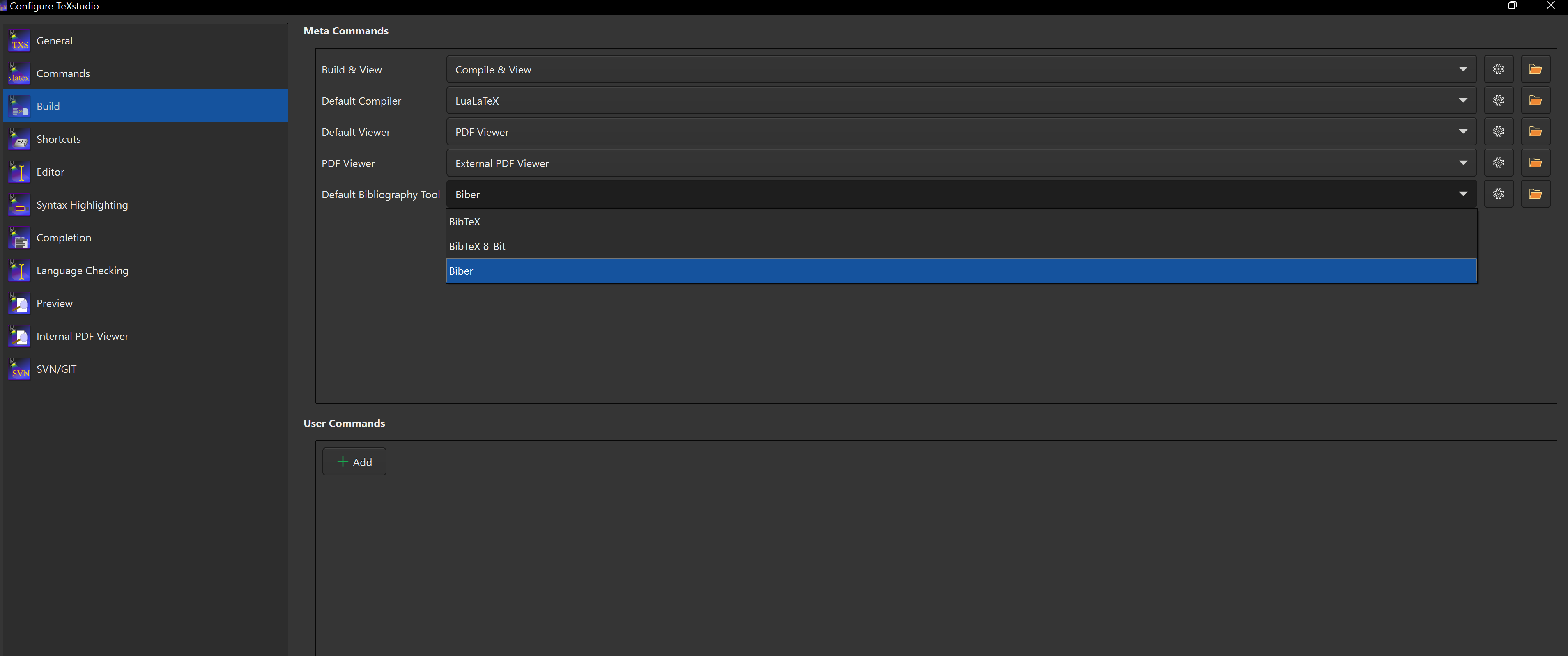
Reference Databases (BiBTeX)
Reference databases are normally referred to as BiBTeX
files, and have the extension .bib. They contain one or
more entries, one for each reference, and within each are a series of
fields.
Create a new file in your project called
sample-references.bib and add the following content:
BIBTEX
@article{Thomas2008,
author = {Thomas, Christine M.},
title = {The Fascinating World of Penguins},
journal = {Penguin Chronicles},
date = {2008},
pages = {7009-7024},
}
@book{Graham1995,
author = {Graham, Richard L. and Harris, Lisa A.},
title = {The Humble Paperclip},
subtitle = {Master of the Modern Office},
publisher = {Scranton Press},
year = {1995},
}This is an example of a BiBTeX file that contains a reference for an
article and another for a book. Each entry type starts with a the
@ symbol, followed by the type of the referencing item
(e.g. article) and all information appears within a pair of
curly braces {}.
The various fields are given in key-value format. Exactly which fields you need to give depends on the type of entry.
You might notice that in the author field, surname and
givenname and each entry (author) is separated by the word
and. This is essential: the format of the output needs to
know which author is which. When using biblatex this
applies also to the fields publisher and
location, in which you can also have many values.
You might also notice that in the article title, some entries are in an extra set of braces. This is to prevent any case-changing that might be applied to the title.
The BibTeX Format
Editing BiBTeX files by hand can be difficult and tedious. A number of tools exist to help you manage your reference files. You can find a list of sugggested tools in the references section.
For the purposes of this workshop, we’ll use biblatex,
but feel free to explore other options (e.g. natbib) on
your own.
There are many different bibliography styles available, and you can find a list of them at CTAN. Check if one of those bibligraphy and citation styles meets your requirements. If you want to finetune an existing one we suggest to take a look at biblatex-ext.
Challenges
Challenge 1: Add another reference, then delete it.
Try adding the following reference to your
sample-references.bib file:
BIBTEX
@book{Huff1954,
author = {Huff, Darrell},
title = {How to Lie with Statistics},
publisher = {W. W. Norton \& Company},
year = {1954},
}Then, add a citation to this reference in your document. Try a couple different styles of citation commands. Then, once you have it working, delete the reference and re-compile your document. What happens?
You might expect removing the reference to either error or remove the citation from the text, but it doesn’t - instead we get a placeholder in the text and a warning in the log. A missing reference is not so critical an error that we can’t render the document, but we should probably fix it.
Challenge 2: What’s wrong with this?
We have the following reference in our document:
BIBTEX
@misc{mikolov2013,
title ={Efficient Estimation of Word Representations in Vector Space},
author ={Mikolov, Tomas and Chen, Kai and Corrado, Greg and Dean, Jeffrey},
year ={2013},
eprint ={1301.3781},
archivePrefix ={arXiv},
primaryClass ={cs.CL},
url ={https://arxiv.org/abs/1301.3781},
}We are using biblatex to manage our references, and we
identify this reference in the text like this:
When we compile our document, we see the following error:
OUTPUT
The Word2Vec algorithm (mikolov) is a popular method for generating word embeddings.What’s wrong with this reference? How can we fix it?
We are referencing the key mikolov in our document, but
the key in our BiBTeX file is mikolov2013. We need to
update our citation command to \autocite{mikolov2013}. Note
that LaTeX still compiles the document, but it gives us a warning that
the reference is missing and uses the key as a placeholder. You might
use this to temporarily mark a reference that you haven’t added yet,
just be sure to clear all of your warnings before finializing your
document.
Challenge 3: What’s problem with this?
We inculde the following reference in our document:
BIBTEX
@article{bentham2011,
author = {H. Muller, Rainer and Shegokar, Ranjita and M. Keck, Cornelia},
title = {20 Years of Lipid Nanoparticles (SLN & NLC): Present State of Development & Industrial Applications},
journal= {Current Drug Discovery Technologies},
year = {2011},
volume = {8},
number = {3},
pages = {207--227},
doi = {https://doi.org/10.2174/157016311796799062},
publisher = {Bentham Science Publishers},
}We are using biblatex and cite this reference in the
text as follows:
What happens when compiling this document? What is wrong with the reference, and how can it be fixed?
The issue in this reference is cause by a sepcial character
(& in the title field). In LaTeX the ampersand
& is reserved for alignment, so it must be escaped
(\&)in normal text.
If special characters are not escaped properly, LaTeX produce
unexpected output or may fail to compile. In some cases, this can also
corrupt auxiliary files (such as .aux or
.bbl), preventing the document from rendering as expected.
If problems persist after correcting the reference, a common solution is
to delete all intermediate files and recompile the document from
scratch. Deleting them forces a clean rebuild.
Corrected bib entry:
BIBTEX
@article{bentham2011,
author = {H. Muller, Rainer and Shegokar, Ranjita and M. Keck, Cornelia},
title = {20 Years of Lipid Nanoparticles (SLN \& NLC): Present State of Development \& Industrial Applications},
journal= {Current Drug Discovery Technologies},
year = {2011},
volume = {8},
number = {3},
pages = {207--227},
doi = {https://doi.org/10.2174/157016311796799062},
publisher = {Bentham Science Publishers},
}- References are stored in a reference database, seperate from the LaTeX document.
- BiBTeX files are used to store references in a processing-friendly
format and have the extension
.bib. - There are multiple libraries available to manage references in LaTeX
documents, including
natbibandbiblatex. - We can use the
\citecommand or one of its variants to cite references in our document.
Content from Context Sensitive Quotations
Last updated on 2025-07-16 | Edit this page
Overview
Questions
- How can I semantically markup quotes so they adapt to language and style?
- What is the benefit of letting
csquotesintegrate withbiblatexfor quoting? - How do I switch between different quotation styles (e.g. English “…” vs. German „…“)?
- How can I automatically hyphenate and nest quotations correctly in another language?
Objectives
By the end of this lesson, learners will be able to:
- Explain the difference between inline quotes, block quotes, and semantic quoting.
- Use
\enquote{…}(and its variants) to produce context‑sensitive quotation marks. - Reference a quoted passage with a citation that feeds into the bibliographic list.
- Switch quote styles to match locale conventions (e.g. German vs. English).
- Configure
csquotesto handle nested quotes, foreign‑language quotes, and hyphenation.
Introduction
Quotations play an essential role in scholarly writing, allowing you
to bring in authoritative voices or preserve precise wording. But “dumb”
straight ASCII quotes ("like this") don’t adapt to language
conventions, and block quotes can be cumbersome to format manually.
The csquotes package makes all of this
automatic:
- It defines semantic commands like
\enquote{…}, which insert the right opening/closing marks based on the current language (e.g. “English style,” ‹French guillemets›, or „German quotes“). - It integrates smoothly with
biblatex, so you can attach a citation to a quote with\blockquote[prenote][postnote]{…}and have the entry appear in your bibliography. - It handles nested quotations, switching automatically to secondary marks (e.g. single quotes) when you nest quotes.
- It can load language-specific hyphenation patterns so that breaking long quoted passages doesn’t lead to poorly shaped lines.
Before we begin, make sure you’ve installed
csquotes:
and that your document preamble loads it (ideally after the package
biblatex):
Various Types of Quotation
Inline Quotes
Instead of typing this by hand:
you write:
-
\enquote{…}uses the main quote style. -
\enquote*{…}(star form) forces the inner quote style, even if not nested.
Here is a full example.
Text or Block Quotes
For longer quotations you can use:
LATEX
\blockquote[see Hoare 1973, p. 195]{%
Documentation must be regarded as an integral part of the process of design and coding.
A good programming language will encourage and assist the programmer to write clear,
self-documenting code, and even perhaps to develop and display a pleasant style of writing.%
}- The optional bracket is a postnote (e.g. source or page number).
It will produce an indented block and automatically insert quotation
marks (or omit them, depending on style). There is also the
\textquote-command but this is ommitted since
\blockquote has the greater flexibility.
Referencing Source of Quote to BibLaTeX-Entry
One of the biggest advantages of using csquotes is its
interplay with biblatex as a way of referencing sources. To
use this kind of quotes you also need to have the package
biblatex loaded in your preamble.
BIBTEX
@InCollection{Hoare1973,
author = {Charles Antony Richard Hoare},
title = {Hints on programming language design},
editor = {C. Bunyan},
booktitle = {Computer Systems Reliability},
series = {State of the Art Report},
number = {20},
pages = {193--216},
year = {1973},
url = {http://flint.cs.yale.edu/cs428/documentation/HintsPL.pdf},
urlyear = {2018},
comment = {Documentation must be regarded as an integral part of the process of design and coding. A good programming language will encourage and assist the programmer to write clear, self-documenting code, and even perhaps to develop and display a pleasant style of writing.}
}- ⟨prenote⟩: optional text before the citation (e.g. “see”, “cf.”).
- ⟨postnote⟩: optional locator such as a page number (e.g. “193–216”).
-
⟨key⟩: the BibLaTeX entry key
(e.g.
Hoare1973). - ⟨punct⟩: punctuation inserted inside the closing quote (e.g. a comma or period).
- ⟨text⟩: the quoted passage itself.
- ⟨tpunct⟩: punctuation inserted after the closing quote (e.g. a period or question mark).
Here is an example:
LATEX
\blockcquote[see][195]{Hoare1973}{Documentation must be regarded as an integral part of the process of design and coding. A good programming language will encourage and assist the programmer to write clear, self-documenting code, and even perhaps to develop and display a pleasant style of writing.}This will produce (with default settings for
biblatex):
Documentation must be regarded as an integral part of the process of design and coding. A good programming language will encourage and assist the programmer to write clear, self-documenting code, and even perhaps to develop and display a pleasant style of writing. [see 1, p. 195]
and automatically add the Hoare1973 entry to your
bibliography when you run \printbibliography.
Challenge 1: Referencing Sources
- Add a new entry to your
references.bibfor a short article. - Use
\textcquoteand\blockcquoteto insert a two sentence quote with a pre- and postnote pointing to the entry you just created. Do you see a difference when you use\textcquoteor\blockcquote?
With default settings, quotes written with \blockcquote
will be displayed in the same way as \textcquote. As soon
as the text is longer than three complete lines of text, then the whole
quote is indented and set as a block.
Foreign Language Quotes
csquotes can detect and adjust for foreign passages if
you load polyglossia or babel. For
example:
LATEX
\usepackage[ngerman,english]{babel}
\usepackage[autostyle]{csquotes}
% In your document:
\foreignquote{german}{Er ist der Beste.}This switches to German quotes („…“) only for that passage, then returns to the main language.
You can also nest foreign quotes:
…which might render as (setting in your preamble
\usepackage[autostyle,french=guillemets]{csquotes}): >
“He said, « Je ne sais quoi », before leaving.”
There is also the command \foreignblockcquote that first
needs the language as mandatory argument, for a concrete example:
LATEX
\foreignblockcquote{german}[vgl.][195 (eigene Übersetzung)]{Hoare1973}{%
Die Dokumentation muss als integraler Bestandteil des Entwurfs- und Kodierungsprozesses betrachtet werden. Eine gute Programmiersprache wird den Programmierer ermutigen und unterstützen, klaren, selbstdokumentierenden Code zu schreiben und vielleicht sogar einen angenehmen Schreibstil zu entwickeln und zu pflegen.%
}Auxiliary Commands
When quoting text in a formal way, any changes applied to the quoted
material—such as omissions, insertions, or deletions—should be
explicitly marked. The csquotes package provides three
auxiliary commands for this purpose:
-
\textelp{}/\textelp{⟨text⟩}/\textelp*{⟨text⟩}Prints an ellipsis to indicate omitted material. With an argument, it also shows inserted text in brackets. The starred form reverses insertion order. -
\textins{⟨text⟩}/\textins*{⟨text⟩}Marks added text in square brackets. The starred variant is intended for small modifications (e.g. capitalization). -
\textdel{⟨text⟩}Indicates deletion by printing empty brackets; the omitted text itself is not displayed.
LATEX
She said, “To be, or not to be\textelp{} that is the question.”
He corrected it to “To be, or not to be\textelp{ indeed}\textelp*{ indeed}.”
Old form: “colour” → “colou\textdel{r}”
Insersion: “The quick \textins{brown} fox.”Challenge 2: Auxiliary Commands
- Take the sentence: “The quick brown fox jumps over the lazy dog.”
- Omit the word “brown” using
\textelp{}and show the result. - Insert the word “agile” before “fox” using
\textins{}. - Delete the “s” in “jumps” using
\textdel{}.
Adjust Default Settings
Change the amount of lines you want to have for a block quote:
Adjust the appearance of a deleted word.
Define the way of a source is displayed after the blockquote:
This will put the references in a footnote.
- Use
\enquote{…}for semantic, language-aware inline quotes. - Use
\blockquote{…}for automatic block formatting and citation. - Integrate with
biblatexinside quotes for full bibliographic support. - Switch quote styles per language with
\foreign(c)quote. - Customize nesting, spacing, and thresholds to match publisher or style-guide requirements.
Content from Structuring Sources
Last updated on 2025-07-16 | Edit this page
Overview
Questions
- How can we make it easier to manage large LaTeX projects?
- How can we reuse parts of our LaTeX document in other documents?
- How can we structure our LaTeX project?
Objectives
- Learn how to use commands to include other files in your LaTeX document
- Restructure a LaTeX project to use multiple files
Project Structure
So far, we’ve been putting all of our LaTeX code into a single document. This is fine for small projects, but even with what we have here so far, you might have started to feel like things are getting a little unwieldy and hard to manage.
One of the great things we can do with LaTeX is break our document up into smaller “sources”, which allows us to work on each part of the document separately. You can imagine this might be helpful when working on a large document with multiple chapters, where each chapter is a separate file. You might also find this useful when you intend to reuse parts of your document in other documents, like title pages, tables of contents, or lists of figures.
This also helps with collaboration, as multiple people can work on different parts of the document at the same time without having to worry about conflicts.
Commands
There are two important commands to know when working with multiple sources:
\input{filename}\include{filename}
The \input{filename} command will include the contents
of the file filename.tex at the point where the command is
called as though it was typed directly into the main document. This can
be useful for things that are not, for example, separate chapters, but
rather things like a title page, a table of contents, or a list of
figures.
The \include{filename} command will do the same thing,
but it will also start a new page before including the file. This is
useful for including separate chapters or sections of your document.
When you use \include{filename} you can also use
\includeonly{filename1,filename2} in your preamble. This
will then only insert the file mentioned but respect all other files
regarding e.g. pagenumber, references etc.
Note that in case you have deleted all your *.aux-files
and want to compile from scratch, make sure you have disabled the
\includeonly{}-command. At least for the first run.
Otherwise the other files that are included will not be known to the
compiler and therefor omitted. This has consequences for references,
page numbers etc.
Input Example
Let’s try out using the \input{filename} command. We’ll
create a new file called input_example.tex in our project
directory with the following contents:
LATEX
\cmd{Input} is useful for including things as if they were typed directly into the main document.
Things like commands don't have to be defined in the included file, as long as they are defined in
the main document.Then, in our main.tex document, let’s add the following
section:
When we compile our document, we should see the contents of
input_example.tex included in our main document.
Include Example
Let’s try out using the \include{filename} command.
We’ll create a new file called include_example.tex in our
project directory with the following contents:
LATEX
\cmd{Include} is useful for including things as if they were typed directly into the main document,
but it will also start a new page before including the file.Then, in our main.tex document, let’s add the following
section:
When we compile our document, we should see the contents of
include_example.tex, however this time the content will
have included a new page before the content.
Another important thing to note about the
\include{filename} command is that it cannot contain
another \include{} command - this will result in an
error.
You can, however, use \input{} inside an
\include{} command or an \input{} command
inside another \input{} command.
Updating Our Project
Now that we’ve seen how to use the \input{filename} and
\include{filename} commands, let’s refactor our project to
use them. We’ll take each section and put it in it’s own file, then
include the files in our main.tex document. This will main
our main document easier to read and manage, while separating out the
content into more manageable pieces.
Let’s also organize our files a little bit. Instead of putting everything in the “root” directory of this project, we’ll create a folder called “content” and put our section files in there.
Separating Our Sections
Let’s make files in our “content” directory for each of our sections:
content/sections.texcontent/lists.texcontent/graphics.texcontent/tables.texcontent/cross-references.texcontent/mathematics.texcontent/fonts-formatting-and-spacing.texcontent/reference-databases.tex
We’ll move the content from each section into the corresponding file.
content/lists.tex
LATEX
\section{Lists}
There are two types of lists: ordered and unordered.
\subsection{Ordered}
Ordered lists do not have numbers associated with each item.
\begin{enumerate}
\item Item 1
\item Item 2
\item Item 3
\end{enumerate}
\subsection{Unordered}
Unordered lists are just a series of items preceded by a marker.
\begin{itemize}
\item Item 1
\item Item 2
\item Item 3
\end{itemize}content/graphics.tex
LATEX
\section{Graphics}
We can include \kw{images} in our document using the \cmd{graphicx} package, which lets us use the
\cmd{includegraphics} command.
\includegraphics{figures/example-image.png}
\subsection{Small Image}
We can pass parameters to the \cmd{includegraphics} command to adjust the appearance of the image.
\includegraphics[height=2cm]{figures/example-image.png}
Other possible options include:
\begin{itemize}
\item width: the width of the image
\item scale: the scaling factor of the image
\item angle: the angle of rotation of the image
\item clip: whether to clip the image to its bounding box
\item trim: trim the image by a specified amount
\item draft: display a box instead of the image
\end{itemize}
\subsection{Centered Image}
By placing the \cmd{includegraphics} command inside a center environment, we can center the
image on the page.
\begin{center}
\includegraphics[height=2cm]{figures/example-image.png}
\end{center}
\subsection{Floating Image}
\kw{Floating images} can move around the page as text is added or removed. We can use the
\cmd{figure}environment to create a floating image.
\begin{figure}[ht]
\centering
\includegraphics[height=2cm]{figures/example-image.png}
\end{figure}
Control the position of a floating image by passing paratmeters to the \cmd{figure} environment:
\begin{itemize}
\item h: Place the float "here" (where it appears in the code)
\item t: Place the float at the "top" of the page
\item b: Place the float at the "bottom" of the page
\item p: Place the float on a "page" by itself
\end{itemize}
\subsection{Caption}
We can add a \kw{caption} to our floating image by using the \cmd{caption} command inside of the
\cmd{figure} environment.
\begin{figure}[h]
\centering
\includegraphics[height=2cm]{figures/example-image.png}
\caption{This is a caption for our image.}
\end{figure}content/tables.tex
LATEX
\section{Tables}
\kw{Tables} are defined using the \cmd{tabular} environment.
\input{tables/basic-table}
\subsection{Tables with Horizontal Lines}
We can use the \cmd{\textbackslash toprule}, \cmd{\textbackslash midrule}, and
\cmd{\textbackslash bottomrule} commands from the \cmd{booktabs} package to create horizontal
lines in our table.
\input{tables/table-with-horizontal-lines}
\subsection{Partial Horizontal Lines}
The \cmd{\textbackslash cmidrule} command can be used to create partial horizontal lines in a
table. The command accepts the arguments {number-number}, where the first number is the column to
start the line and last number is the column to end the line.
\input{tables/table-with-partial-horizontal-lines}
\subsection{Merging Cells}
Merge cells horizontally using the \cmd{\textbackslash multicolumn} command. This command takes
three arguments:
\begin{itemize}
\item The number of cells which should be merged
\item The alignment of the merged cell (l, c, or r)
\item The contents of the merged cell
\end{itemize}
\input{tables/table-with-merged-cells}content/cross-references.tex
LATEX
\section{Cross References}
\label{sec:cross-references}
\subsection{Material for the Introduction}
In this section, we introduce two new concepts:
\begin{tabular}{cp{9cm}}
Command & Description \\
\toprule
\kw{label} & Marks a spot in the document \\
\kw{ref} & Refers to a marked spot in the document \\
\bottomrule
\label{tab:cross-reference-commands}
\end{tabular}
We can \kw{refer} to the section with the \cmd{ref} command, like this: \ref{sec:cross-references}.
We can likewise refer to the table like this: \ref{tab:cross-reference-commands}.content/mathematics.tex
LATEX
\section{Mathematics}
There are two kinds of math mode in LaTeX: inline and display. Inline math mode is marked with
a pair of dollar signs, whereas display math mode is marked with a pair of square brackets.
\subsection{Inline Math Mode}
The Pythagorean theorem is $a^2 + b^2 = c^2$.
\subsection{Display Math Mode}
The Fourier Transform is defined as:
\[
\hat{f}(\xi) = \int_{-\infty}^\infty f(x) e^{-2\pi i \xi x} \, dx
\]
Where:
\begin{itemize}
\item \( f(x) \) is the function we are transforming,
\item \( \hat{f}(\xi) \) is the Fourier Transform of \( f(x) \),
\item \( \xi \) is the frequency variable,
\item \( i \) is the imaginary unit.
\end{itemize}
\subsection{Math in Environments}
The quadratic formula is:
\begin{equation}
x = \frac{-b \pm \sqrt{b^2 - 4ac}}{2a}
\label{eq:quadratic}
\end{equation}
This will allow us to refer to the equation later in the document with \cmd{ref} like this:
Refer to Equation \ref{eq:quadratic}.
\subsection{The `amsmath` Package}
Solve the following recurrence for $ n,k\geq 0 $:
\[
Q_{n,0} = 1 \quad Q_{0,k} = [k=0];
\]
\[
Q_{n,k} = Q_{n-1,k}+Q_{n-1,k-1}+\binom{n}{k}, \quad\text{for $n$, $k>0$.}
\]content/reference-databases.tex
LATEX
\section{Reference Databases}
One of the best features of LaTeX when writing academic documents is the ability to easily and
confidently \kw{cite references}.
We can cite the article by Thomas (e.g. with `\textbackslash autocite\{Thomas2008\}`) and it will show up in the references.
You should see that the citation appears in the text (`(Thomas et al. 2008)`), and the reference
now appears at the end of the document. \cmd{\textbackslash autocite} is a command that automatically chooses the
citation style for you.
Some additional commands that are available in `biblatex`:
\begin{itemize}
\item `\textbackslash cite\{key\}` or `\textbackslash cite\{key1, key2\}`: Cite the reference with the given key
\item `\textbackslash cites\{key1\}\{key2\}\{key-n\}`: Cite multiple references.
\item `\textbackslash usepackage\{\}\textbackslash parentcite\{key\}`: Cite the parent reference of the given key.
\item `\textbackslash autocite\{key\}`: Automatically choose the citation style.
\item `\textbackslash smartcite\{key\}`: Automatically choose the citation style, but with more control.
\item `\textbackslash footcite\{key\}`: Cite the reference in a footnote.
\end{itemize}
A plain citation looks like this \cite{Graham1995}, while multiple citations look like this
\cites{Graham1995}[see][p. 42]{Thomas2008}. We already used autocite, but we can also use the
similar smartcite \smartcite{Graham1995}. The benefit with smartcite is that you
can setup that e.g. all references should go into a footnote. You can continue
using smartcite when you are *in* a footnote and it will then detect that there
is no need for creating another footnote but behaving like autocite.Then, in our main.tex document, we’ll include each of
these files using the \input{filename}:
LATEX
\include{content/sections}
\include{content/lists}
\include{content/graphics}
\include{content/tables}
\include{content/cross-references}
\include{content/mathematics}
\include{content/fonts-formatting-and-spacing}
\include{content/reference-databases}Note that the \include{filename} command does not
require the .tex extension. LaTeX will assume that the file
is a .tex file if no extension is provided.
This is also true for someof the other commands we’ve seen, such as
\includegraphics{}. It is personal preference whether you
include the extension or not.
When we compile our document, we should see the same content as before, but now we can make changes in our content files, and the changes will be reflected in our main document.
Other Files
While we’re at it, let’s also create files for our packages, commands, and title page. We’ll also put these into their own directory called “preamble”:
preamble/packages.texpreamble/custom-commands.texpreamble/titlepage.tex
Our New main.tex
Our main.tex document should now look like this:
LATEX
% This command tells LaTeX what kind of document we are creating (article).
\documentclass{article}
\input{preamble/packages}
\input{preamble/custom-commands}
\addbibresource{sample-references.bib}
% Everything before the \begin{document} command is called the preamble.
\begin{document} % The document body starts here
\include{content/titlepage}
Hello World!
This is my first \kw{LaTeX} document.
\include{content/sections}
\include{content/lists}
\include{content/graphics}
\include{content/tables}
\include{content/cross-references}
\include{content/mathematics}
\include{content/fonts-formatting-and-spacing}
\include{content/reference-databases}
\printbibliography
\end{document}Note that we still need to put the content in the appropriate order.
For example, you can’t add \input{includes/packages} at the
end of the document, as it needs to be included before the document
starts.
Challenges
Challenge 1: Refactor the rest of the document
We started with a couple of files, but see if you can refactor the rest of the document.
The soultion to this challenge is in the section above.
Challenge 2: Refactor Your Document with Multiple Files
Refactor the following LaTeX document to use multiple files.
LATEX
% This is the main document: main.tex
\documentclass{article}
\begin{document}
\begin{titlepage}
    \centering
    \huge
    \textbf{My Custom LaTeX Title Page}

    \vspace{1cm} % Space between title and subtitle
    \normalsize
    \textit{A Sample Document with Custom Formatting}

    \vfill % Fill remaining space
    \large
    January 1, 2025
\end{titlepage}
\section{Tables}
\begin{tabular}{lll}
Fruit & Quantity & Price \\
Apple & 5 & 1.50 \\
Banana & 6 & 2.00 \\
Orange & 4 & 1.20 \\
\end{tabular}
\section{Graphics}
\begin{figure}[ht]
\centering
\includegraphics[height=2cm]{example-image.PNG}
\caption{This is a caption for our image.}
\end{figure}
\end{document}- Separate the content into different files for the sections by
tables.texandgraphics.tex. - Organize the file for the titlepage in a folder named “includes” and
name the file
titlepage.tex. - Organize the files for tables and graphics in a folder named “content”.
- Use the
\inputcommand to include the titlepage and the content in yourmain.texdocument.
LATEX
% This is the main document: main.tex

\documentclass{article}


\begin{document}

% Include title page
\input{includes/titlepage}

% Include content from different files in the "content" folder
\input{content/sections}
\input{content/lists}
\input{content/graphics}
\input{content/tables}
\input{content/cross-references}
\input{content/math}
\input{content/text-and-spacing}

\end{document}
Challenge 3: Why did we do this?
In our content/tables.tex file, we have a bunch of
\input{} commands for the tables instead of writing the
tables directly in the file. Why did we do this? What is the benefit of
doing this?
Using an \input command inserts the table contents
directly into the document as though it was typed, which means that we
can reuse the same table in multiple documents without having to copy
paste it. For example, if we were making a presentation in LaTeX, we
could use the same table in our presentation. This means that if we make
a change to the table, it will be reflected in all of the documents in
which we use it.
(This reflects the programming principle of “Don’t Repeat Yourself” (DRY)!)
Challenge 4: Restructuring a larger document?
There isn’t a specific correct answer for this challenge, but one idea might be something that looks like this:
├── main.tex
├── preamble.tex
├── refereces.bib
├── content/
│   ├── introduction.tex
│   ├── model_architecture.tex
│   ├── model_results.tex
│   └── conclusion.tex
├── tables/
└── model_results.tex- LaTeX projects can contain many files that reference each other
- The
\input{filename}and\include{filename}commands allow you to include the contents of other files in your document - The
\frontmatter,\mainmatter,\backmatter, and\appendixcommands help structure your document
Content from Loading and Manipulating Data
Last updated on 2026-04-08 | Edit this page
Overview
Questions
- Why would I want to load data into my LaTeX document?
- How can I incorporate data analysis into my LaTeX document?
Objectives
- Load a csv file into a LaTeX document and display it as a table
- Manipulate the data to get summary statistics in another table
- Create a simple plot using the data
Introduction
To start with we need to use the datatool package. We
can find information about the package on CTAN: https://ctan.org/pkg/datatool,
including a readme.
We can install the package using the following command in the terminal:
We can then load the package in our LaTeX document using the following command:
We’ll also need some data to work with. We’ll use some simple CSVs that contain data about GDP per capita and life expectancy from the past 50 years. You can download the data from this website. Unzip the file and place the contents in you project directory.
Your directory should look like this:
project/
├── data
│   ├── gapminder_tidy.csv
│   ├── gapminder_gdp_africa.csv
│   ├── gapminder_gdp_americas.csv
│   ├── gapminder_gdp_asia.csv
│   ├── gapminder_gdp_europe.csv
│   └── gapminder_gdp_oceania.csv
├── main.tex
├── other files...
Loading Data
First things first, we want to load the data into our LaTeX document.
We can do this with the \DTLread command from the
datatool package. This command takes two arguments: the
name of the database and the path to the CSV file.
LATEX
\section{Loading and Manipulating Data}

We are using the datatool package to load and manipulate data in our LaTeX document.

\subsection{Loading Data}

We can \kw{load} the data from the CSV file with the \cmd{DTLread} command:

\DTLread[name=gapminder]{data/gapminder_tidy_oceania.csv}
You’ll notice that loading the data doesn’t display any output in the document. We need a seperate command to show the data.
Displaying Data
We can display the data in a table using the
\DTLdisplaydb command. This command takes the name of the
database as an argument and displays the data in a table.
Your document should now look something like this:
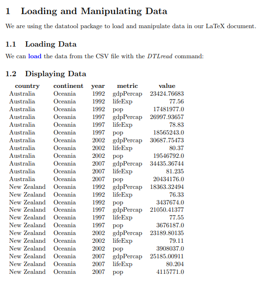
We can see the data now, but we have way too much data to show in a single table. Let’s filter the data to only show the GDP per capita data.
Filtering Data
We can filter the data by using the \DTLforeach command.
This command iterates over all the rows of our database and does
something with each row (like a for loop in programming languages). We
can also add conditions to the first argument to filter the data. We can
use \DTLisieq to check if a value in the row is equal to a
specific value.
Note that this command has a few more arguments than the previous one:
- The first argument is a list of conditions to filter the data.
- The second argument is the name of the database.
- The third argument is a list of variables to extract from the
database.
- Note that all variables you use in the
\DTLforeachcommand must be identified here.
- Note that all variables you use in the
- The last argument is the code to execute for each row that matches the conditions.
LATEX
\subsection{Filtering Data}

\DTLforeach[
  \DTLisieq{\year}{2002}
  \and
  \DTLisieq{\metric}{gdpPercap}
]{gapminder}{
  \country=country,
  \year=year,
  \metric=metric,
  \datavalue=value%
}{
  \country\,(\year): \datavalue\\
}You’ll notice that the “value” variable is assigned to
\datavalue and not \value. This is because
\value is a reserved command in LaTeX, so we need to use a
different name for the variable.
Your filtered data should look something like this:
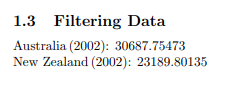
Data Aggregation
A very common task in data analysis might be to aggregate the data
and calculate some sort of summary statistic. For this,
datatool provides some usefule commands:
\DTLsumforkeys\DTLmaxforkeys\DTLmeanforkeys\DTLsdforkeys
We can use these commands to calculate the sum, maximum, mean, and
standard deviation of a variable for a specific set of keys. The syntax
is (Almost!) identical to the \DTLforeach command.
Note that compared to the \DTLforeach command, the
second and third arguments are switched. In this command, the second
argument is the list of variables and the third argument is the database
name.
Creating New Datasets
The \DTLforeach command is extremely useful - say we
want to create a new dataset to work with that only contains the GDP per
capita data for the year 2002 for our dataset. We could filter the
original dataset each time and then perform our analysis, but this could
be inefficient and it could be complicated.
Instead, let’s use some new command to create a new dataset that only contains the data we want to work with:
LATEX
\subsection{Creating New Datasets}

\DTLnewdb{filteredgapminder}

\DTLforeach[
  \DTLisieq{\year}{2002}
  \and
  \DTLisieq{\metric}{gdpPercap}
]{gapminder}{
  \country=country,
  \year=year,
  \metric=metric,
  \datavalue=value
}{
  \DTLnewrow{filteredgapminder}
  \dtlexpandnewvalue% https://tex.stackexchange.com/a/375856/98739
  \DTLnewdbentry{filteredgapminder}{country}{\country}
  \DTLnewdbentry{filteredgapminder}{value}{\datavalue}
}
Some things to point out here:
- We first create a new database with the
\DTLnewdbcommand. This creates a new database in memory we can add rows to later.
- We then use the
\DTLnewrowcommand to create a new row in the database.
- We use the
\DTLnewdbentrycommand to add a new entry to the row. The first argument is the name of the database, the second argument is the name of the column, and the third argument is the value to add to that column.
We need to use the \dtlexpandnewvalue command otherwise
the data will not be expanded, meaning the compiler cannot read the
content of the variable used.
We can now display the new database using the
\DTLdisplaydb command:
Your document should now look something like this:
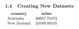
Plotting Data
Now that we have our filtered data, we can also plot it!. We’ll need
a new package for this called databar, so add this to your
preamble:
Now we can use the \DTLBarChart command to create a bar
chart from our data:
LATEX
\subsection{Plotting Data}

\DTLbarchart
{
  variable=\datavalue,
}{filteredgapminder}{
  \datavalue=value,
  \country=country
}Your document should now look something like this:

Challenge 1: Changing the Input Data
There are other data files in the data directory. Try
switching out the gapminder_tidy_oceania.csv file for one
of the other files and see if this code still works.
Did you notice anything different? If so, what was it?
If you used one of the other files, you might have noticed that the
time it took create the pdf was much longer. This is because the other
files contain more data than the gapminder_tidy_oceania.csv
file. The datatool package can handle large datasets, but
it can take a long time to process them.
You might consider pre-processing the data in another language (like R or Python) and then loading the processed data into your LaTeX document.
Challenge 2: Diplaying the results in a table
In the “Data Filtering” section above, we displayed the filtered data
using the \DTLforeach command like this:
LATEX
\DTLforeach[%
  \DTLisieq{\year}{2002}
  \and
  \DTLisieq{\metric}{gdpPercap}
]{gapminder}{%
  \country=country,
  \year=year,
  \metric=metric,
  \datavalue=value%
}{
  \country\,(\year): \datavalue\\
}
How might you display the results in a table? See if you can get the output to look like this:
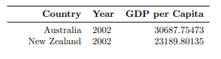
Refer back to the Episode on Tables to review the syntax for creating tables in LaTeX.
NOTE: There is an issue with datatool and
\bottomrule in tables - for now, skip the
\bottomrule command in your table. (You’ll get an error
about “misplaced ”.)
\begin{tabular}{rlr}
\toprule
\textbf{Country} & \textbf{Year} & \textbf{GDP per Capita} \\
\midrule
\DTLforeach[
  \DTLisieq{\year}{2002}
  \and
  \DTLisieq{\metric}{gdpPercap}
]{gapminder}{%
  \country=country,
  \year=year,
  \metric=metric,
  \datavalue=value%
}{
  \country & \year & \datavalue\\
}%
\end{tabular}- The
datatoolpackage allows us to load and manipulate data in LaTeX documents. - We can load data from a CSV file using the
\DTLreadcommand. - We can display data in a table using the
\DTLdisplaydbcommand. - We can filter data using the
\DTLforeachcommand and conditions. - We can aggregate data using commands like
\DTLmeanforkeys,\DTLsumforkeys, etc.
Content from Documentation and Finding Help
Last updated on 2026-04-09 | Edit this page
Overview
Questions
- Where can I find help for writing LaTeX documents?
- How do I find out what commands a package provides?
Objectives
- Learn how to find help for LaTeX documents
CTAN (The Comprehensive TeX Archive Network)
A large number of LaTeX packages are available on CTAN. CTAN contains packages and related documentation for many widely used LaTeX packages. You can search the archive for specific strings, or browse by category.
 Project pages
Individual package pages often contain links to detailed documentation, including PDF manuals and example files. Additional you can find links to the package’s source code, and information about the author(s) and ratings from other users.
Texdoc
Texdoc provides a modern interface for looking up package documentation. Much like CTAN, you can search for packages and view their documentation.
Texdoc is also available as a command line tool, which queries the same database of information, but allows you to search for packages and documentation from the command line.
Other Resources
As with any language there are many other resources that you can make use of. The Stack Exchange for LaTeX is a great place to ask questions and find answers to common problems.
Challenges
Challenge 1: Find it in the documentation!
We have the geometry package loaded in our document, and we know we want to use to to set the margins of the document, but we want to set them to 2cm on the left and right, and 4cm on the top and bottom. We also want to set the page size to A4. Can you find the documentation for the command and see how to do this?
Challenge 2: Find a specific package.
We have a very particular document we want to create - we are talking about specific positions on a chess board and we want to render these directly in the document. Can you find a package that will help us do this? Can you make a simple chess board using this package?
Searching either CTAN or Texdoc for “chess” will return a number of
packages. We’ll use the chessboard package for our example.
To make a simple chess board, we can use the chessboard
command:
- CTAN is a large archive of LaTeX packages and documentation
- Texdoc is a website & command line tool for searching LaTeX documentation