Loading and Manipulating Data
Last updated on 2026-04-08 | Edit this page
Overview
Questions
- Why would I want to load data into my LaTeX document?
- How can I incorporate data analysis into my LaTeX document?
Objectives
- Load a csv file into a LaTeX document and display it as a table
- Manipulate the data to get summary statistics in another table
- Create a simple plot using the data
Introduction
To start with we need to use the datatool package. We
can find information about the package on CTAN: https://ctan.org/pkg/datatool,
including a readme.
We can install the package using the following command in the terminal:
We can then load the package in our LaTeX document using the following command:
We’ll also need some data to work with. We’ll use some simple CSVs that contain data about GDP per capita and life expectancy from the past 50 years. You can download the data from this website. Unzip the file and place the contents in you project directory.
Your directory should look like this:
project/
├── data
│   ├── gapminder_tidy.csv
│   ├── gapminder_gdp_africa.csv
│   ├── gapminder_gdp_americas.csv
│   ├── gapminder_gdp_asia.csv
│   ├── gapminder_gdp_europe.csv
│   └── gapminder_gdp_oceania.csv
├── main.tex
├── other files...
Loading Data
First things first, we want to load the data into our LaTeX document.
We can do this with the \DTLread command from the
datatool package. This command takes two arguments: the
name of the database and the path to the CSV file.
LATEX
\section{Loading and Manipulating Data}

We are using the datatool package to load and manipulate data in our LaTeX document.

\subsection{Loading Data}

We can \kw{load} the data from the CSV file with the \cmd{DTLread} command:

\DTLread[name=gapminder]{data/gapminder_tidy_oceania.csv}
You’ll notice that loading the data doesn’t display any output in the document. We need a seperate command to show the data.
Displaying Data
We can display the data in a table using the
\DTLdisplaydb command. This command takes the name of the
database as an argument and displays the data in a table.
Your document should now look something like this:
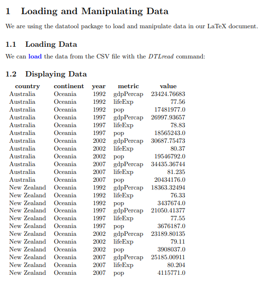
We can see the data now, but we have way too much data to show in a single table. Let’s filter the data to only show the GDP per capita data.
Filtering Data
We can filter the data by using the \DTLforeach command.
This command iterates over all the rows of our database and does
something with each row (like a for loop in programming languages). We
can also add conditions to the first argument to filter the data. We can
use \DTLisieq to check if a value in the row is equal to a
specific value.
Note that this command has a few more arguments than the previous one:
- The first argument is a list of conditions to filter the data.
- The second argument is the name of the database.
- The third argument is a list of variables to extract from the
database.
- Note that all variables you use in the
\DTLforeachcommand must be identified here.
- Note that all variables you use in the
- The last argument is the code to execute for each row that matches the conditions.
LATEX
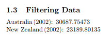
\subsection{Filtering Data}

\DTLforeach[
  \DTLisieq{\year}{2002}
  \and
  \DTLisieq{\metric}{gdpPercap}
]{gapminder}{
  \country=country,
  \year=year,
  \metric=metric,
  \datavalue=value%
}{
  \country\,(\year): \datavalue\\
}You’ll notice that the “value” variable is assigned to
\datavalue and not \value. This is because
\value is a reserved command in LaTeX, so we need to use a
different name for the variable.
Your filtered data should look something like this:
Data Aggregation
A very common task in data analysis might be to aggregate the data
and calculate some sort of summary statistic. For this,
datatool provides some usefule commands:
\DTLsumforkeys\DTLmaxforkeys\DTLmeanforkeys\DTLsdforkeys
We can use these commands to calculate the sum, maximum, mean, and
standard deviation of a variable for a specific set of keys. The syntax
is (Almost!) identical to the \DTLforeach command.
Note that compared to the \DTLforeach command, the
second and third arguments are switched. In this command, the second
argument is the list of variables and the third argument is the database
name.
Creating New Datasets
The \DTLforeach command is extremely useful - say we
want to create a new dataset to work with that only contains the GDP per
capita data for the year 2002 for our dataset. We could filter the
original dataset each time and then perform our analysis, but this could
be inefficient and it could be complicated.
Instead, let’s use some new command to create a new dataset that only contains the data we want to work with:
LATEX
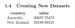
\subsection{Creating New Datasets}

\DTLnewdb{filteredgapminder}

\DTLforeach[
  \DTLisieq{\year}{2002}
  \and
  \DTLisieq{\metric}{gdpPercap}
]{gapminder}{
  \country=country,
  \year=year,
  \metric=metric,
  \datavalue=value
}{
  \DTLnewrow{filteredgapminder}
  \dtlexpandnewvalue% https://tex.stackexchange.com/a/375856/98739
  \DTLnewdbentry{filteredgapminder}{country}{\country}
  \DTLnewdbentry{filteredgapminder}{value}{\datavalue}
}
Some things to point out here:
- We first create a new database with the
\DTLnewdbcommand. This creates a new database in memory we can add rows to later. - We then use the
\DTLnewrowcommand to create a new row in the database. - We use the
\DTLnewdbentrycommand to add a new entry to the row. The first argument is the name of the database, the second argument is the name of the column, and the third argument is the value to add to that column.
We need to use the \dtlexpandnewvalue command otherwise
the data will not be expanded, meaning the compiler cannot read the
content of the variable used.
We can now display the new database using the
\DTLdisplaydb command:
Your document should now look something like this:
Plotting Data
Now that we have our filtered data, we can also plot it!. We’ll need
a new package for this called databar, so add this to your
preamble:
Now we can use the \DTLBarChart command to create a bar
chart from our data:
LATEX
\subsection{Plotting Data}

\DTLbarchart
{
  variable=\datavalue,
}{filteredgapminder}{
  \datavalue=value,
  \country=country
}Your document should now look something like this:

Challenge 1: Changing the Input Data
There are other data files in the data directory. Try
switching out the gapminder_tidy_oceania.csv file for one
of the other files and see if this code still works.
Did you notice anything different? If so, what was it?
If you used one of the other files, you might have noticed that the
time it took create the pdf was much longer. This is because the other
files contain more data than the gapminder_tidy_oceania.csv
file. The datatool package can handle large datasets, but
it can take a long time to process them.
You might consider pre-processing the data in another language (like R or Python) and then loading the processed data into your LaTeX document.
Challenge 2: Diplaying the results in a table
In the “Data Filtering” section above, we displayed the filtered data
using the \DTLforeach command like this:
LATEX
\DTLforeach[%
\DTLisieq{\year}{2002}
\and
\DTLisieq{\metric}{gdpPercap}
]{gapminder}{%
\country=country,
\year=year,
\metric=metric,
\datavalue=value%
}{
\country\,(\year): \datavalue\\
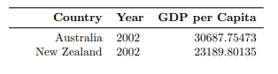
}How might you display the results in a table? See if you can get the output to look like this:
Refer back to the Episode on Tables to review the syntax for creating tables in LaTeX.
NOTE: There is an issue with datatool and
\bottomrule in tables - for now, skip the
\bottomrule command in your table. (You’ll get an error
about “misplaced ”.)
\begin{tabular}{rlr}
\toprule
\textbf{Country} & \textbf{Year} & \textbf{GDP per Capita} \\
\midrule
\DTLforeach[
  \DTLisieq{\year}{2002}
  \and
  \DTLisieq{\metric}{gdpPercap}
]{gapminder}{%
  \country=country,
  \year=year,
  \metric=metric,
  \datavalue=value%
}{
  \country & \year & \datavalue\\
}%
\end{tabular}- The
datatoolpackage allows us to load and manipulate data in LaTeX documents. - We can load data from a CSV file using the
\DTLreadcommand. - We can display data in a table using the
\DTLdisplaydbcommand. - We can filter data using the
\DTLforeachcommand and conditions. - We can aggregate data using commands like
\DTLmeanforkeys,\DTLsumforkeys, etc.