Unsupervised methods - Clustering

Estimated time: 60 minutes

Overview

Questions

• What is unsupervised learning?
• How can we use clustering to find data points with similar attributes?

Objectives

• Understand the difference between supervised and unsupervised learning.
• Identify clusters in data using k-means clustering.
• Understand the limitations of k-means when clusters overlap.
• Use spectral clustering to overcome the limitations of k-means.

Unsupervised learning

---

In episode 2 we learnt about supervised learning. Now it is time to explore unsupervised learning.

Sometimes we do not have the luxury of using labelled data. This could be for a number of reasons:

• We have labelled data, but not enough to accurately train our model
• Our existing labelled data is low-quality or innacurate
• It is too time-consuming to (manually) label more data
• We have data, but no idea what correlations might exist that we could model!

In this case we need to use unsupervised learning. As the name suggests, this time we do not “supervise” the ML algorithm by providing it labels, but instead we let it try to find its own patterns in the data and report back on any correlations that it might find. You can think of unsupervised learning as a way to discover labels from the data itself.

Clustering

---

Clustering is the grouping of data points which are similar to each other. It can be a powerful technique for identifying patterns in data. Clustering analysis does not usually require any training and is therefore known as an unsupervised learning technique. Clustering can be applied quickly due to this lack of training.

Applications of clustering

---

• Looking for trends in data
• Reducing the data around a point to just that point (e.g. reducing colour depth in an image)
• Pattern recognition

K-means clustering

---

The k-means clustering algorithm is a simple clustering algorithm that tries to identify the centre of each cluster. It does this by searching for a point which minimises the distance between the centre and all the points in the cluster. The algorithm needs to be told how many k clusters to look for, but a common technique is to try different numbers of clusters and combine it with other tests to decide on the best combination.

Callout

Hyper-parameters again

‘K’ is also an exmaple of a hyper-parameter for the k-means clustering technique. Another example of a hyper-parameter is the N-degrees of freedom for polynomial regression. Keep an eye out for others throughout the lesson!

K-means with Scikit-Learn

To perform a k-means clustering with Scikit-Learn we first need to import the sklearn.cluster module.

PYTHON

import sklearn.cluster as skl_cluster

For this example, we’re going to use Scikit-Learn’s built-in ‘random data blob generator’ instead of using an external dataset. Therefore we’ll need the sklearn.datasets.samples_generator module.

PYTHON

import sklearn.datasets as skl_datasets

Now lets create some random blobs using the make_blobs function. The n_samples argument sets how many points we want to use in all of our blobs while cluster_std sets the standard deviation of the points. The smaller this value the closer together they will be. centers sets how many clusters we’d like. random_state is the initial state of the random number generator. By specifying this value we’ll get the same results every time we run the program. If we don’t specify a random state then we’ll get different points every time we run. This function returns two things: an array of data points and a list of which cluster each point belongs to.

PYTHON

import matplotlib.pyplot as plt

# Lets define a plotting function for ourselves.
def plot_clusters(data, labels, centers=None):
    tx = data[:, 0]
    ty = data[:, 1]
    fig = plt.figure(1, figsize=(4, 4))
    plt.scatter(tx, ty, edgecolor='k', c=labels)
    if centers is not None:
        for cluster_x, cluster_y in centers:
            plt.scatter(cluster_x, cluster_y, s=150, c='white', edgecolor='k', linewidths=1.5, marker='X')
    plt.show()

Lets create the clusters.

PYTHON

data, cluster_id = skl_datasets.make_blobs(n_samples=400, cluster_std=0.75, centers=4, random_state=1)
plot_clusters(data, cluster_id)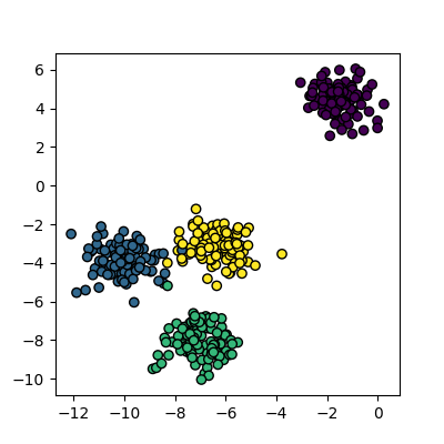

Plot of the random clusters

Now that we have some data we can try to identify the clusters using k-means. First, we need to initialise the KMeans module and tell it how many clusters to look for. Next, we supply it with some data via the fit function, in much the same way we did with the regression functions earlier on. Finally, we run the predict function to find the clusters.

PYTHON

Kmean = skl_cluster.KMeans(n_clusters=4)
Kmean.fit(data)
clusters = Kmean.predict(data)

The data can now be plotted to show all the points we randomly generated. To make it clearer which cluster points have been classified we can set the colours (the c parameter) to use the clusters list that was returned by the predict function. The Kmeans algorithm also lets us know where it identified the centre of each cluster. These are stored as a list called ‘cluster_centers_’ inside the Kmean object. Let’s plot the points from the clusters, colouring them by the output from the K-means algorithm, and also plot the centres of each cluster as a red X.

plot_clusters(data, clusters, Kmean.cluster_centers_)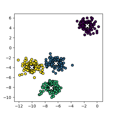

Plot of the fitted random clusters

Here is the code all in a single block.

PYTHON

import sklearn.cluster as skl_cluster
import sklearn.datasets as skl_datasets
import matplotlib.pyplot as plt

data, cluster_id = skl_datasets.make_blobs(n_samples=400, cluster_std=0.75, centers=4, random_state=1)

Kmean = skl_cluster.KMeans(n_clusters=4)
Kmean.fit(data)
clusters = Kmean.predict(data)

plot_clusters(data, clusters, Kmean.cluster_centers_)

Callout

Working in multiple dimensions

Although this example shows two dimensions, the kmeans algorithm can work in more than two. It becomes very difficult to show this visually once we get beyond 3 dimensions. Its very common in machine learning to be working with multiple variables and so our classifiers are working in multi-dimensional spaces.

Limitations of k-means

• Requires number of clusters to be known in advance
• Struggles when clusters have irregular shapes
• Will always produce an answer finding the required number of clusters even if the data isn’t clustered (or clustered in that many clusters)
• Requires linear cluster boundaries

An example of kmeans failing on non-linear cluster boundaries

Advantages of k-means

• Simple algorithm and fast to compute
• A good choice as the first thing to try when attempting to cluster data
• Suitable for large datasets due to its low memory and computing requirements

Challenge

Exercise: K-Means with overlapping clusters

Adjust the program above to increase the standard deviation of the blobs (the cluster_std parameter to make_blobs) and increase the number of samples (n_samples) to 4000. You should start to see the clusters overlapping.

Do the clusters that are identified make sense? Is there any strange behaviour?

Show me the solution

Increasing n_samples to 4000 and cluster_std to 3.0 looks like this:

Kmeans attempting to classify overlapping clusters

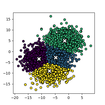
The straight line boundaries between clusters look a bit strange.

Challenge

Exercise: How many clusters should we look for?

Using k-means requires us to specify the number of clusters to expect. A common strategy to get around this is to vary the number of clusters we are looking for.

Modify the code you wrote in the previous exercise to loop through searching for between 2 and 10 clusters of 400 points. Which (if any) of the results look more sensible? What criteria might you use to select the best one? Try increasing the number of centers to 6. If you didn’t know this value, how would you select the best number of clusters?

Show me the solution

PYTHON

data, cluster_id = skl_datasets.make_blobs(n_samples=400, cluster_std=3, centers=6, random_state=1)
for cluster_count in range(2,11):
    Kmean = skl_cluster.KMeans(n_clusters=cluster_count)
    Kmean.fit(data)
    clusters = Kmean.predict(data)
    plot_clusters(data, clusters, Kmean.cluster_centers_)

We of course know ahead of time that there are 6 centers, but imagine if we didn’t. You might find some of the clusters more sensible than others but there is no real way to know which one is best.

Data in the wild is unlikely to be as neat and tidy as the examples here, so it’s good to keep in mind that there may not be a single clear ‘right answer’ when it comes to clustering.

DBSCAN

---

Disadvanges of K-means

Kmeans seems to work pretty well for our contrived example of blobs of data, but let’s look at exactly why it struggles with irregular clusters. For the next section, we’ll use the make_moons function to generate our data. This will create two interleaving half circles.

PYTHON

data, cluster_id = skl_datasets.make_moons(n_samples=400, noise=0.1, random_state=1)
plot_clusters(data, cluster_id)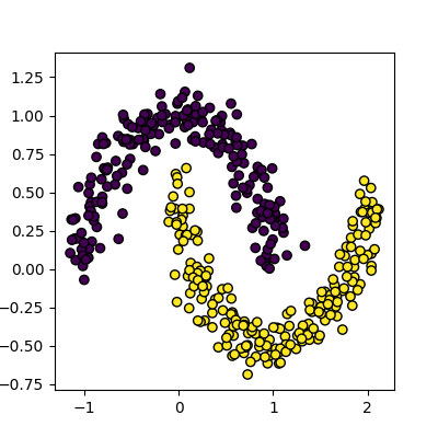

Next, let’s try to use Kmeans on this data the same way we did before.

PYTHON

Kmean = skl_cluster.KMeans(n_clusters=2)
Kmean.fit(data)
clusters = Kmean.predict(data)
plot_clusters(data, clusters, Kmean.cluster_centers_)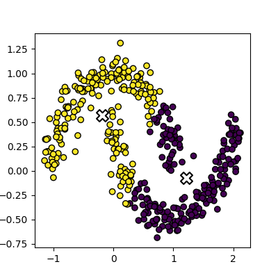

This is an example of exactly what we mean when we say that k-means struggles with irregular clusters. The clusters are not circular in nature, and there is no straight line that can be drawn to separate them. Luckily, there’s another method we can use to cluster this data…

DBSCAN clustering

DBSCAN stands for Density Based Spatial Clustering of Applications with Noise. The general concept is that it looks for clusters of data that are closely packed together, and marks points that are far away from any cluster as noise.

The algorithm is iterative, and works like this:

• Define a radius (eps) and a minimum number of points (min_samples) to form a cluster
• For each point
  • Find all points within a specified radius (eps)
    • If a point has more than min_samples neighbors, it is a core point and starts/expands a cluster
    • If a point has fewer than min_samples neighbors, it is a border point and is added to the nearest cluster
    • If a point has no neighbors, it is marked as noise
  • Points that are not core or border points are considered noise

Compared to K-means, this method has several advantages:

• we are able to identify a cluster of arbitrary shape, as membership in a cluster is determined by proximity to the other points of the cluster, rather than proximity to a central point.
• We can identify noise points that do not belong to any cluster, which can be useful for outlier detection.
• We do not need to specify the number of clusters in advance, as the algorithm will find as many clusters as there are dense regions in the data.

Let’s try it out on our data:

PYTHON

dbscan = skl_cluster.DBSCAN(min_samples=5, eps=0.18)
dbscan.fit(data)
plot_clusters(data, dbscan.labels_)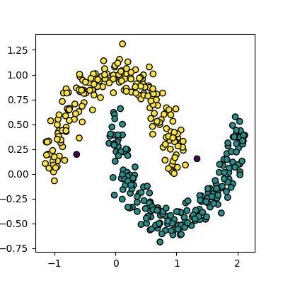

Disadvantages of DBSCAN

DBSCAN isn’t perfect though, and has some disadvantages:

• It can struggle to identify clusters in data with varying densities, as the eps and min_samples parameters are global and may not be suitable for all clusters.
• It can be sensitive to the choice of eps and min_samples parameters, which can be difficult to select without prior knowledge of the data.
• It can struggle with high-dimensional data, as the concept of density becomes less meaningful in high-dimensional spaces.

Callout

Selecting Hyper-parameters for DBSCAN

For low dimensionality data, min_samples is commonly set to 5. A general rule of thumb for high dimensionality data is to set min_samples to 2 * number of dimensions.

The eps parameter can be selected by plotting the k-distance graph, which shows the distance to the k-th nearest neighbor for each point in the dataset. The value of eps can be chosen as the distance at which there is a significant change in the slope of the graph, indicating a transition from dense to sparse regions of the data.

We can create a k-distance graph from our data like this:

PYTHON

from sklearn.neighbors import NearestNeighbors
import numpy as np

k = 5  # min_samples for DBSCAN
nearest_neighbors = NearestNeighbors(n_neighbors=k).fit(data)
distances, _ = nearest_neighbors.kneighbors(data)

k_distances = np.sort(distances[:, k - 1])[::-1]

plt.plot(k_distances)
plt.xlabel("Points")
plt.ylabel(f"{k}-NN Distance")
plt.title("k-Distance")
plt.axhline(y=0.18, color='r', linestyle='--')
plt.show()

Spectral clustering

---

Spectral clustering is a technique that attempts to overcome the linear boundary problem of k-means clustering. It works by treating clustering as a graph partitioning problem and looks for nodes in a graph with a small distance between them. See this introduction to spectral clustering if you are interested in more details about how spectral clustering works.

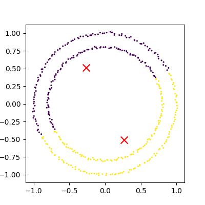
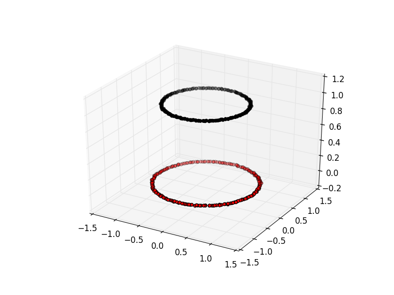
Here is an example of spectral clustering on two concentric circles:

Spectral clustering on two concentric circles

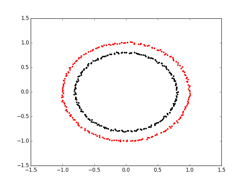
Spectral clustering uses something called a ‘kernel trick’ to introduce additional dimensions to the data. A common example of this is trying to cluster one circle within another (concentric circles). A k-means classifier will fail to do this and will end up effectively drawing a line which crosses the circles. However spectral clustering will introduce an additional dimension that effectively moves one of the circles away from the other in the additional dimension. This does have the downside of being more computationally expensive than k-means clustering.

Spectral clustering viewed with an extra dimension

Spectral clustering with Scikit-Learn

Lets try out using Scikit-Learn’s spectral clustering. To make the concentric circles in the above example we need to use the make_circles function in the sklearn.datasets module. This works in a very similar way to the make_blobs function we used earlier on.

PYTHON

import sklearn.datasets as skl_data

circles, circles_clusters = skl_data.make_circles(n_samples=400, noise=.01, random_state=0)
plot_clusters(circles, circles_clusters)

The code for calculating the SpectralClustering is very similar to the kmeans clustering, but instead of using the sklearn.cluster.KMeans class we use the sklearn.cluster.SpectralClustering class.

PYTHON

model = skl_cluster.SpectralClustering(n_clusters=2, affinity='nearest_neighbors', assign_labels='kmeans')

The SpectralClustering class combines the fit and predict functions into a single function called fit_predict.

PYTHON

labels = model.fit_predict(circles)
plot_clusters(circles, labels)

Here is the whole program combined with the kmeans clustering for comparison. Note that this produces two figures. To view both of them use the “Inline” graphics terminal inside the Python console instead of the “Automatic” method which will open a window and only show you one of the graphs.

PYTHON

import sklearn.cluster as skl_cluster
import sklearn.datasets as skl_data

circles, circles_clusters = skl_data.make_circles(n_samples=400, noise=.01, random_state=0)

# cluster with kmeans
Kmean = skl_cluster.KMeans(n_clusters=2)
Kmean.fit(circles)
clusters = Kmean.predict(circles)

# plot the data, colouring it by cluster
plot_clusters(circles, clusters, Kmean.cluster_centers_)

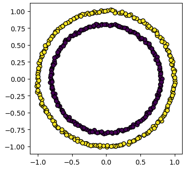
# cluster with spectral clustering
model = skl_cluster.SpectralClustering(n_clusters=2, affinity='nearest_neighbors', assign_labels='kmeans')
labels = model.fit_predict(circles)
plot_clusters(circles, labels)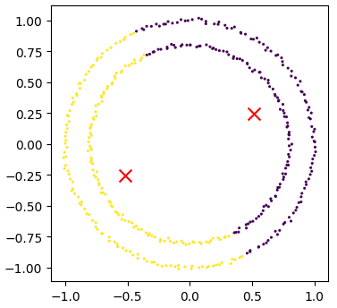

Kmeans attempting to cluster the concentric circles

Spectral clustering on the concentric circles

Challenge

Comparing k-means and spectral clustering performance

Modify the program we wrote in the previous exercise to use spectral clustering instead of k-means and save it as a new file.

Time how long both programs take to run. Add the line import time at the top of both files as the first line, and get the start time with start_time = time.time().

End the program by getting the time again and subtracting the start time from it to get the total run time. Add end_time = time.time() and print("Elapsed time:",end_time-start_time,"seconds") to the end of both files.

Compare how long both programs take to run generating 4,000 samples and testing them for between 2 and 10 clusters. - How much did your run times differ? - How much do they differ if you increase the number of samples to 8,000? - How long do you think it would take to compute 800,000 samples (estimate this, it might take a while to run for real)?

Show me the solution

KMeans version: runtime around 4 seconds (your computer might be faster/slower)

PYTHON

import matplotlib.pyplot as plt
import sklearn.cluster as skl_cluster
from sklearn.datasets import make_blobs
import time

start_time = time.time()
data, cluster_id = make_blobs(n_samples=4000, cluster_std=3,
                                       centers=4, random_state=1)

for cluster_count in range(2,11):
    Kmean = skl_cluster.KMeans(n_clusters=cluster_count)
    Kmean.fit(data)
    clusters = Kmean.predict(data)

    plt.scatter(data[:, 0], data[:, 1], s=15, linewidth=0, c=clusters)
    plt.title(str(cluster_count)+" Clusters")

plt.show()
end_time = time.time()
print("Elapsed time = ", end_time-start_time, "seconds")

Spectral version: runtime around 9 seconds (your computer might be faster/slower)

import matplotlib.pyplot as plt
import sklearn.cluster as skl_cluster
from sklearn.datasets import make_blobs
import time

start_time = time.time()
data, cluster_id = make_blobs(n_samples=4000, cluster_std=3,
                                       centers=4, random_state=1)

for cluster_count in range(2,11):
    model = skl_cluster.SpectralClustering(n_clusters=cluster_count,
                                       affinity='nearest_neighbors',
                                       assign_labels='kmeans')
    labels = model.fit_predict(data)

    plt.scatter(data[:, 0], data[:, 1], s=15, linewidth=0, c=labels)
    plt.title(str(cluster_count)+" Clusters")
plt.show()
end_time = time.time()
print("Elapsed time = ", end_time-start_time, "seconds")

When the number of points increases to 8000 the runtimes are 24 seconds for the spectral version and 5.6 seconds for kmeans.

The runtime numbers will differ depending on the speed of your computer, but the relative difference should be similar.

For 4000 points kmeans took 4 seconds, while spectral took 9 seconds. A 2.25 fold difference.

For 8000 points kmeans took 5.6 seconds, while spectral took 24 seconds. A 4.28 fold difference. Kmeans is 1.4 times slower for double the data, while spectral is 2.6 times slower.

The relative difference is diverging. If we used 100 times more data we might expect a 100 fold divergence in execution times.

Kmeans might take a few minutes while spectral will take hours.

Key Points

• Clustering is a form of unsupervised learning.
• Unsupervised learning algorithms don’t need training.
• Kmeans is a popular clustering algorithm.
• Kmeans is less useful when one cluster exists within another, such as concentric circles.
• Spectral clustering can overcome some of the limitations of Kmeans.
• Spectral clustering is much slower than Kmeans.
• Scikit-Learn has functions to create example data.