Supervised methods - Regression

Estimated time: 120 minutes

Overview

Questions

• What is supervised learning?
• What is regression?
• How can I model data and make predictions using regression methods?

Objectives

• Apply linear regression with Scikit-Learn to create a model.
• Measure the error between a regression model and input data.
• Analyse and assess the accuracy of a linear model using Scikit-Learn’s metrics library.
• Understand how more complex models can be built with non-linear equations.
• Apply polynomial modelling to non-linear data using Scikit-Learn.

Supervised learning

---

Classical machine learning is often divided into two categories – supervised and unsupervised learning.

For the case of supervised learning we act as a “supervisor” or “teacher” for our ML algorithms by providing the algorithm with “labelled data” that contains example answers of what we wish the algorithm to achieve.

For instance, if we wish to train our algorithm to distinguish between images of cats and dogs, we would provide our algorithm with images that have already been labelled as “cat” or “dog” so that it can learn from these examples. If we wished to train our algorithm to predict house prices over time we would provide our algorithm with example data of datetime values that are “labelled” with house prices.

Supervised learning is split up into two further categories: classification and regression. For classification the labelled data is discrete, such as the “cat” or “dog” example, whereas for regression the labelled data is continuous, such as the house price example.

In this episode we will explore how we can use regression to build a “model” that can be used to make predictions.

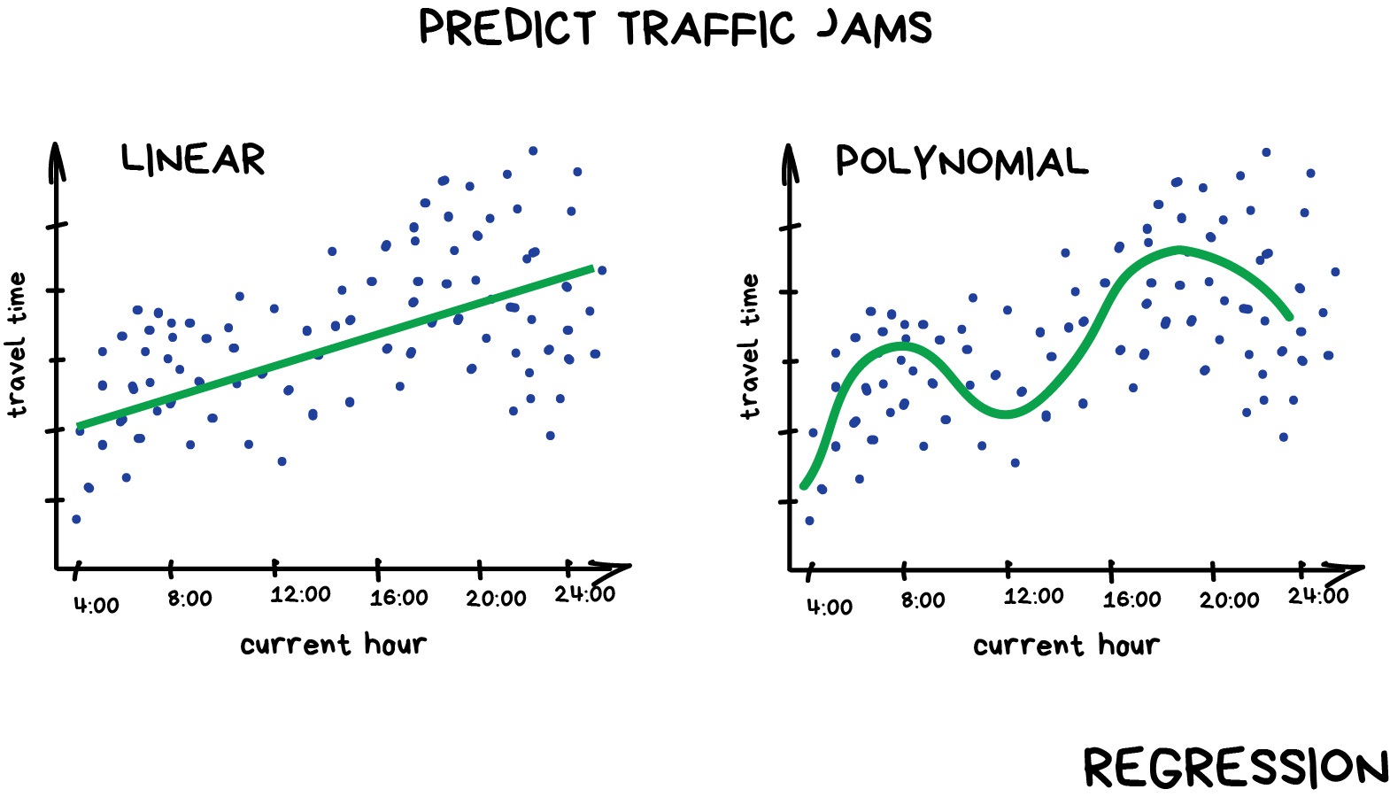
Regression

---

Regression is a statistical technique that relates a dependent variable (a label in ML terms) to one or more independent variables (features in ML terms). A regression model attempts to describe this relation by fitting the data as closely as possible according to mathematical criteria. This model can then be used to predict new labelled values by inputting the independent variables into it. For example, if we create a house price model we can then feed in any datetime value we wish, and get a new house price value prediction.

Regression can be as simple as drawing a “line of best fit” through data points, known as linear regression, or more complex models such as polynomial regression, and is used routinely around the world in both industry and research. You may have already used regression in the past without knowing that it is also considered a machine learning technique!

Example of linear and polynomial regressions

Linear regression using Scikit-Learn

We’ve had a lot of theory so time to start some actual coding! Let’s create regression models for a small bundle of datasets known as Anscombe’s Quartet. These datasets are available through the Python plotting library Seaborn. Let’s define our bundle of datasets, extract out the first dataset, and inspect it’s contents:

Instructor Note

Francis Anscombe was a statistician who created a set of datasets that all have the same basic statistical properties, such as means and standard deviations, but which look very different when plotted. This is a great example of how statistics can be misleading, and why visualising data is important.

PYTHON

import seaborn as sns

# Anscomes Quartet consists of 4 sets of data
data = sns.load_dataset("anscombe")
data.head()

# Split out the 1st dataset from the total
data_1 = data[data["dataset"]=="I"]
data_1 = data_1.sort_values("x")

# Inspect the data
data_1.head()

We see that the dataset bundle has the 3 columns dataset, x, and y. We have already used the dataset column to extract out Dataset I ready for our regression task. Let’s visually inspect the data:

PYTHON

import matplotlib.pyplot as plt

plt.scatter(data_1["x"], data_1["y"])
plt.xlabel("x")
plt.ylabel("y")
plt.show()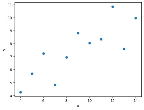

Inspection of our dataset

In this regression example we will create a Linear Regression model that will try to predict y values based upon x values.

In machine learning terminology: we will use our x feature (variable) and y labels(“answers”) to train our Linear Regression model to predict y values when provided with x values.

The mathematical equation for a linear fit is y = mx + c where y is our label data, x is our input feature(s), m represents the gradient of the linear fit, and c represents the intercept with the y-axis.

A typical ML workflow is as following: * Define the model (also known as an estimator) * Tweak your data into the required format for your model * Train your model on the input data * Predict some values using the trained model * Check the accuracy of the prediction, and visualise the result

We’ll define functions for each of these steps so that we can quickly perform linear regressions on our data. First we’ll define a function to pre-process our data into a format that Scikit-Learn can use.

PYTHON

import numpy as np
def pre_process_linear(x, y):
    # sklearn requires a 2D array, so lets reshape our 1D arrays.
    x_data = np.array(x).reshape(-1, 1)
    y_data = np.array(y).reshape(-1, 1)

    return x_data, y_data

Next we’ll define a model, and train it on the pre-processed data. We’ll also inspect the trained model parameters m and c:

PYTHON

from sklearn.linear_model import LinearRegression

def fit_a_linear_model(x_data, y_data):
    # Define our estimator/model
    model = LinearRegression()

    # train our estimator/model using our data
    lin_regress = model.fit(x_data, y_data)

    # inspect the trained estimator/model parameters
    m = lin_regress.coef_
    c = lin_regress.intercept_
    print("linear coefs=", m, c)

    return lin_regress

Then we’ll define a function to make predictions using our trained model, and calculate the Root Mean Squared Error (RMSE) of our predictions:

PYTHON

import math
from sklearn.metrics import mean_squared_error

def predict_linear_model(lin_regress, x_data, y_data):
    # predict some values using our trained estimator/model
    # (in this case we predict our input data!)
    linear_data = lin_regress.predict(x_data)

    # calculated a RMS error as a quality of fit metric
    error = math.sqrt(mean_squared_error(y_data, linear_data))
    print("linear error=", error)

    # return our trained model so that we can use it later
    return linear_data

Instructor Note

The Mean Squared Error (MSE) is a common metric used to measure the quality of a regression model. It calculates the average of the squares of the errors, which are the differences between predicted and actual values. The RMSE is simply the square root of the MSE, and it provides a measure of how far off our predictions are from the actual values in the same units as our labels.

Why not Mean Absolute Error? or Mean Squared Error?

RMSE more heavily penalises large errors, and because we square and then take the root, the value is in the same units as our data, which makes it easier to interpret. It also has nice mathematical properties that make it easier to work with in some cases.

Finally, we’ll define a function to plot our input data, our linear fit, and our predictions:

PYTHON

def plot_linear_model(x_data, y_data, predicted_data):
    # visualise!
    # Don't call .show() here so that we can add extra stuff to the figure later
    plt.scatter(x_data, y_data, label="input")
    plt.plot(x_data, predicted_data, "-", label="fit")
    plt.plot(x_data, predicted_data, "rx", label="predictions")
    plt.xlabel("x")
    plt.ylabel("y")
    plt.legend()

We will be training a few Linear Regression models in this episode, so let’s define a handy function to combine input data processing, model creation, training our model, inspecting the trained model parameters m and c, make some predictions, and finally visualise our data.

PYTHON

def fit_predict_plot_linear(x, y):
    x_data, y_data = pre_process_linear(x, y)
    lin_regress = fit_a_linear_model(x_data, y_data)
    linear_data = predict_linear_model(lin_regress, x_data, y_data)
    plot_linear_model(x_data, y_data, linear_data)

    return lin_regress

Now we have defined our generic function to fit a linear regression we can call the function to train it on some data, and show the plot that was generated:

PYTHON

# just call the function here rather than assign.
# We don't need to reuse the trained model yet
fit_predict_plot_linear(data_1["x"], data_1["y"])

plt.show()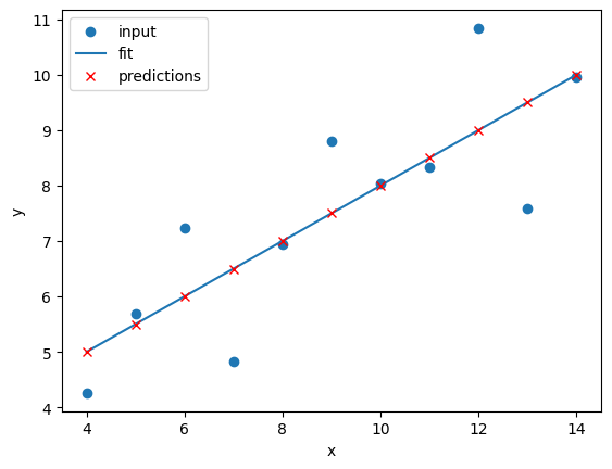

Linear regression of dataset I

This looks like a reasonable linear fit to our first dataset. Thanks to our function we can quickly perform more linear regressions on other datasets.

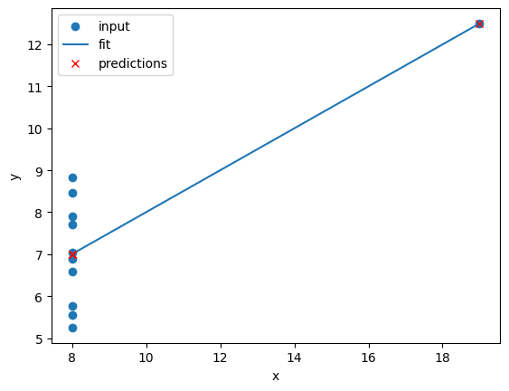
Let’s quickly perform a new linear fit on the 2nd Anscombe dataset:

PYTHON

data_2 = data[data["dataset"]=="II"]
fit_predict_plot_linear(data_2["x"],data_2["y"])

plt.show()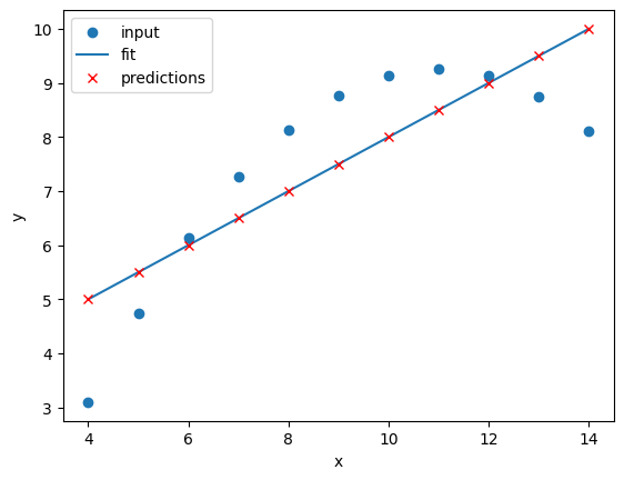

Linear regression of dataset II

It looks like our linear fit on Dataset II produces a nearly identical fit to the linear fit on Dataset I. Although our errors look to be almost identical our visual inspection tells us that Dataset II is probably not a linear correllation and we should try to make a different model.

Challenge

Exercise: Repeat the linear regression excercise for Datasets III and IV.

Adjust your code to repeat the linear regression for the other datasets. What can you say about the similarities and/or differences between the linear regressions on the 4 datasets?

Show me the solution

PYTHON

# Repeat the following and adjust for dataset IV
data_3 = data[data["dataset"]=="III"]
fit_predict_plot_linear(data_3["x"],data_3["y"])
plt.show()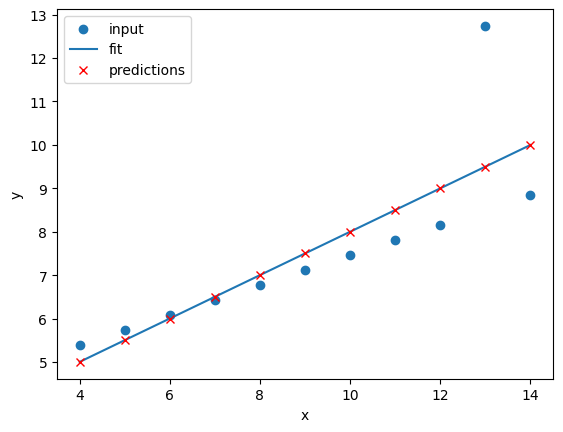

Linear regression of dataset III

Linear regression of dataset IV

The 4 datasets all produce very similar linear regression fit parameters (m and c) and RMSEs despite visual differences in the 4 datasets. This is intentional as the Anscombe Quartet is designed to produce near identical basic statistical values such as means and standard deviations. While the trained model parameters and errors are near identical, our visual inspection tells us that a linear fit might not be the best way of modelling all of these datasets.

Polynomial regression using Scikit-Learn

---

Now that we have learnt how to do a linear regression it’s time look into polynomial regressions. Polynomial functions are non-linear functions that are commonly-used to model data. Mathematically they have N degrees of freedom and they take the following form y = a + bx + cx^2 + dx^3 ... + mx^N

If we have a polynomial of degree N=1 we once again return to a linear equation y = a + bx or as it is more commonly written y = mx + c. Let’s create a polynomial regression using N=2.

In Scikit-Learn this is done in two steps. First we pre-process our input data x_data into a polynomial representation using the PolynomialFeatures function. Then we can create our polynomial regressions using the LinearRegression().fit() function, but this time using the polynomial representation of our x_data.

Instructor Note

PolynomialFeatures is a class in Scikit-Learn that generates polynomial features. We specify a degree, then “fit_transform” our data to create a new feature set that includes all polynomial combinations, so for example PolynomialFeatures(degree=2) will create a new feature set that includes a constant term, the original feature, and the square of the original feature.

PYTHON

from sklearn.preprocessing import PolynomialFeatures

def pre_process_poly(x, y):
    # sklearn requires a 2D array, so lets reshape our 1D arrays.
    x_data = np.array(x).reshape(-1, 1)
    y_data = np.array(y).reshape(-1, 1)

    # create a polynomial representation of our data
    poly_features = PolynomialFeatures(degree=2)
    x_poly = poly_features.fit_transform(x_data)

    return x_poly, x_data, y_data


def fit_poly_model(x_poly, y_data):
    # Define our estimator/model(s)
    poly_regress = LinearRegression()

    # define and train our model
    poly_regress.fit(x_poly, y_data)

    # inspect trained model parameters
    poly_m = poly_regress.coef_
    poly_c = poly_regress.intercept_
    print("poly_coefs", poly_m, poly_c)

    return poly_regress


def predict_poly_model(poly_regress, x_poly, y_data):
    # predict some values using our trained estimator/model
    # (in this case - our input data)
    poly_data = poly_regress.predict(x_poly)

    poly_error = math.sqrt(mean_squared_error(y_data, poly_data))
    print("poly error=", poly_error)

    return poly_data


def plot_poly_model(x_data, poly_data):
    # visualise!
    plt.plot(x_data, poly_data, label="poly fit")
    plt.legend()


def fit_predict_plot_poly(x, y):
    # Combine all of the steps
    x_poly, x_data, y_data = pre_process_poly(x, y)
    poly_regress = fit_poly_model(x_poly, y_data)
    poly_data = predict_poly_model(poly_regress, x_poly, y_data)
    plot_poly_model(x_data, poly_data)

    return poly_regress

Lets plot our input dataset II, linear model, and polynomial model together, as well as compare the errors of the linear and polynomial fits.

PYTHON

# Sort our data in order of our x (feature) values
data_2 = data[data["dataset"] == "II"]
data_2 = data_2.sort_values("x")

fit_predict_plot_linear(data_2["x"], data_2["y"])
fit_predict_plot_poly(data_2["x"], data_2["y"])

plt.show()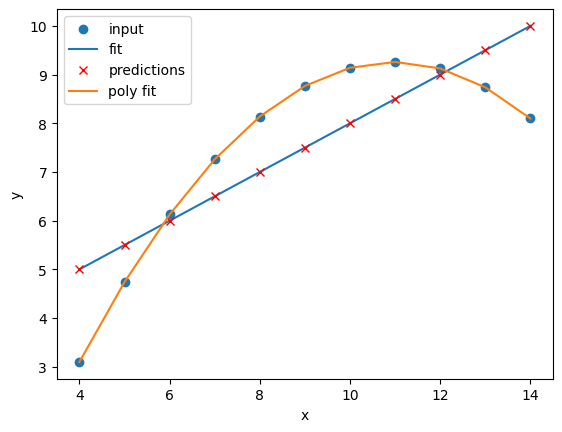

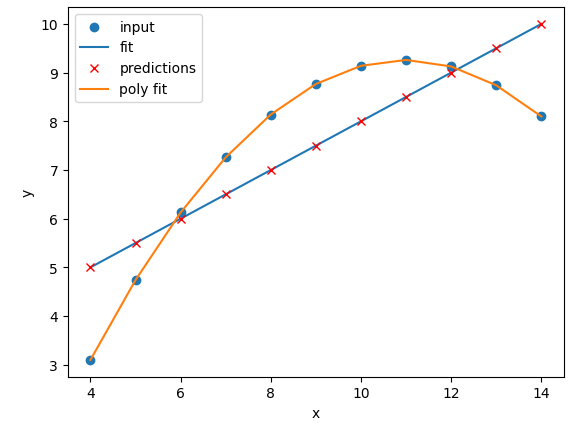
Comparison of the regressions of our dataset

Comparing the plots and errors it seems like a polynomial regression of N=2 is a far superior fit to Dataset II than a linear fit. In fact, it looks like our polynomial fit almost perfectly fits Dataset II… which is because Dataset II is created from a N=2 polynomial equation!

Challenge

Exercise: Perform and compare linear and polynomial fits for Datasets I, II, III, and IV.

Which performs better for each dataset? Modify your polynomial regression function to take N as an input parameter to your regression model. How does changing the degree of polynomial fit affect each dataset?

Show me the solution

PYTHON

for ds in ["I", "II", "III", "IV"]:
    # Sort our data in order of our x (feature) values
    data_ds = data[data["dataset"] == ds]
    data_ds = data_ds.sort_values("x")
    fit_predict_plot_linear(data_ds["x"], data_ds["y"])
    fit_predict_plot_poly(data_ds["x"], data_ds["y"])

    plt.show()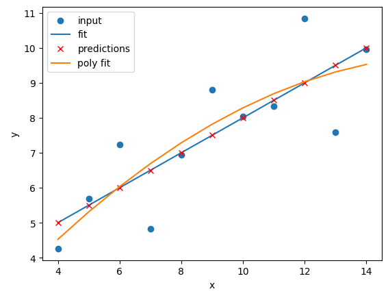

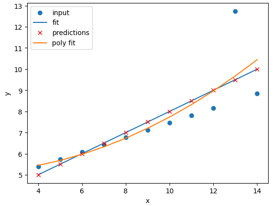
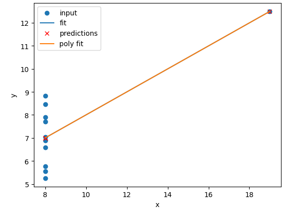
The N=2 polynomial fit is far better for Dataset II. According to the RMSE the polynomial is a slightly better fit for Datasets I and III, however it could be argued that a linear fit is good enough. Dataset III looks like a linear relation that has a single outlier, rather than a truly non-linear relation. The polynomial and linear fits perform just as well (or poorly) on Dataset IV. For Dataset IV it looks like y may be a better estimator of x, than x is at estimating y.

PYTHON

def pre_process_poly(x, y, N):  # <- Add N as an input parameter
    # sklearn requires a 2D array, so lets reshape our 1D arrays.
    x_data = np.array(x).reshape(-1, 1)
    y_data = np.array(y).reshape(-1, 1)

    # create a polynomial representation of our data
    poly_features = PolynomialFeatures(degree=N) # <- Replace 2 with N
    x_poly = poly_features.fit_transform(x_data)

    return x_poly, x_data, y_data

def fit_poly_model(x_poly, y_data):
    # Define our estimator/model(s)
    poly_regress = LinearRegression()

    # define and train our model
    poly_regress.fit(x_poly, y_data)

    # inspect trained model parameters
    poly_m = poly_regress.coef_
    poly_c = poly_regress.intercept_
    print("poly_coefs", poly_m, poly_c)

    return poly_regress

def predict_poly_model(poly_regress, x_poly, y_data):
    # predict some values using our trained estimator/model
    # (in this case - our input data)
    poly_data = poly_regress.predict(x_poly)

    poly_error = math.sqrt(mean_squared_error(y_data, poly_data))
    print("poly error=", poly_error)

    return poly_data


def plot_poly_model(x_data, poly_data, N): # <- Add N as an input parameter
    # visualise!
    plt.plot(x_data, poly_data, label=f"poly fit (N={N})") # <- Add N to the label
    plt.legend()


def fit_predict_plot_poly(x, y, N): # <- Add N as an input parameter
    # Combine all of the steps
    x_poly, x_data, y_data = pre_process_poly(x, y, N) # <- Pass N to pre_process_poly
    poly_regress = fit_poly_model(x_poly, y_data)
    poly_data = predict_poly_model(poly_regress, x_poly, y_data)
    plot_poly_model(x_data, poly_data, N) # <- Pass N to plot_poly_model

    return poly_regress

and a loop to perform polynomial regressions for N=2 to N=10 on each of the datasets:

PYTHON

for ds in ["I", "II", "III", "IV"]:
    # Sort our data in order of our x (feature) values
    data_ds = data[data["dataset"] == ds]
    data_ds = data_ds.sort_values("x")
    fit_predict_plot_linear(data_ds["x"], data_ds["y"])
    for N in range(2, 11):
        print("Polynomial degree =", N)
        fit_predict_plot_poly(data_ds["x"], data_ds["y"], N)
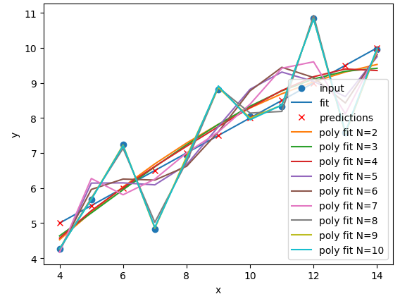
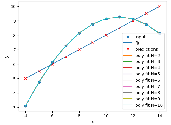
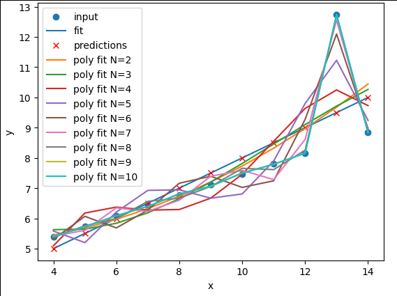
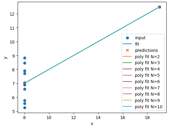
    plt.show()

With a large enough polynomial you can fit through every point with a unique x value. Datasets II and IV remain unchanged beyond N=2 as the polynomial has converged (dataset II) or cannot model the data (Dataset IV). Datasets I and III slowly decrease their RMSE and N is increased, but it is likely that these more complex models are overfitting the data. Overfitting is discussed later in the lesson.

Let’s explore a more realistic scenario

---

Now that we have some convenient Python functions to perform quick regressions on data it’s time to explore a more realistic regression modelling scenario.

Let’s start by loading in and examining a new dataset from Seaborn: a penguin dataset containing a few hundred samples and a number of features and labels.

PYTHON

dataset = sns.load_dataset("penguins")
dataset.head()

We can see that we have seven columns in total: 4 continuous (numerical) columns named bill_length_mm, bill_depth_mm, flipper_length_mm, and body_mass_g; and 3 discrete (categorical) columns named species, island, and sex. We can also see from a quick inspection of the first 5 samples that we have some missing data in the form of NaN values. Let’s go ahead and remove any rows that contain NaN values:

PYTHON

dataset.dropna(inplace=True)
dataset.head()

Now that we have cleaned our data we can try and predict a penguins bill depth using their body mass. In this scenario we will train a linear regression model using body_mass_g as our feature data and bill_depth_mm as our label data. We will train our model on a subset of the data by slicing the first 146 samples of our cleaned data. We will then use our regression function to train and plot our model.

PYTHON

dataset_1 = dataset[:146]

x_data = dataset_1["body_mass_g"]
y_data = dataset_1["bill_depth_mm"]

trained_model = fit_predict_plot_linear(x_data, y_data)

plt.xlabel("mass g")
plt.ylabel("depth mm")
plt.show()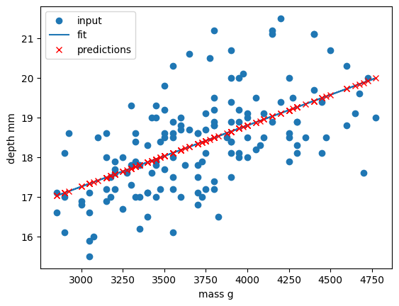

Comparison of the regressions of our dataset

Congratulations! We’ve taken our linear regression function and quickly created and trained a new linear regression model on a brand new dataset. Note that this time we have returned our model from the regression function and assigned it to the variable trained_model. We can now use this model to predict bill_depth_mm values for any given body_mass_g values that we pass it.

Let’s provide the model with all of the penguin samples and visually inspect how the linear regression model performs.

PYTHON

x_data_all, y_data_all = pre_process_linear(dataset["body_mass_g"], dataset["bill_depth_mm"])

y_predictions = predict_linear_model(trained_model, x_data_all, y_data_all)

plt.scatter(x_data_all, y_data_all, label="all data")
plt.scatter(x_data, y_data, label="training data")

plt.plot(x_data_all, y_predictions, label="fit")
plt.plot(x_data_all, y_predictions, "rx", label="predictions")

plt.xlabel("mass g")
plt.ylabel("depth mm")
plt.legend()
plt.show()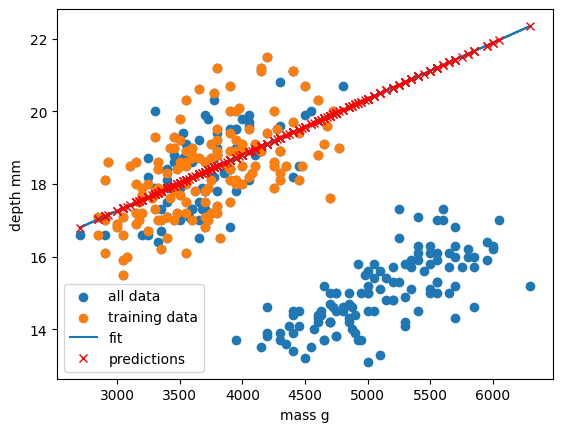

Comparison of the regressions of our dataset

Oh dear. It looks like our linear regression fits okay for our subset of the penguin data, and a few additional samples, but there appears to be a cluster of points that are poorly predicted by our model.

Callout

This is a classic Machine Learning scenario known as over-fitting

We have trained our model on a specific set of data, and our model has learnt to reproduce those specific answers at the expense of creating a more generally-applicable model. Over fitting is the ML equivalent of learning an exam papers mark scheme off by heart, rather than understanding and answering the questions.

Perhaps our model is too simple? Perhaps our data is more complex than we thought? Perhaps our question/goal needs adjusting? Let’s explore the penguin dataset in more depth in the next section!

Key Points

• Scikit-Learn is a Python library with lots of useful machine learning functions.
• Scikit-Learn includes a linear regression function.
• Scikit-Learn can perform polynomial regressions to model non-linear data.